Meteo: Shot-wave incoming radiation (SW_IN) (2006-2024)

Author: Lukas Hörtnagl (holukas@ethz.ch)

Variable

varname = 'SW_IN_T1_47_1'
var = "SW_IN"  # Name shown in plots
units = r"($\mathrm{W\ m^{-2}}$)"

Imports

import importlib.metadata
import warnings
from datetime import datetime
from pathlib import Path
import pandas as pd
import matplotlib.pyplot as plt
import matplotlib.gridspec as gridspec

import diive as dv
from diive.core.io.files import save_parquet, load_parquet
from diive.core.plotting.cumulative import CumulativeYear
from diive.core.plotting.bar import LongtermAnomaliesYear

warnings.filterwarnings(action='ignore', category=FutureWarning)
warnings.filterwarnings(action='ignore', category=UserWarning)
version_diive = importlib.metadata.version("diive")
print(f"diive version: v{version_diive}")

diive version: v0.87.1

Load data

SOURCEDIR = r"../10_METEO"
FILENAME = r"12.3_METEO_GAPFILLED_2004-2024.parquet"
FILEPATH = Path(SOURCEDIR) / FILENAME
df = load_parquet(filepath=FILEPATH)
keeplocs = (df.index.year >= 2006) & (df.index.year <= 2024)
df = df[keeplocs].copy()
df

Loaded .parquet file ..\10_METEO\12.3_METEO_GAPFILLED_2004-2024.parquet (0.060 seconds).
    --> Detected time resolution of <30 * Minutes> / 30min 

	LW_IN_T1_47_1	PA_T1_47_1	PPFD_IN_T1_47_1	RH_T1_47_1	SW_IN_T1_47_1	TA_T1_47_1	SW_IN_T1_47_1_gfXG	TA_T1_47_1_gfXG	PPFD_IN_T1_47_1_gfXG
TIMESTAMP_MIDDLE
2006-01-01 00:15:00	330.969940	92.024002	0.0	98.403702	0.0	1.209000	0.0	1.209000	0.0
2006-01-01 00:45:00	330.439697	91.990997	0.0	98.403702	0.0	1.007000	0.0	1.007000	0.0
2006-01-01 01:15:00	NaN	91.971001	0.0	98.303704	0.0	1.097000	0.0	1.097000	0.0
2006-01-01 01:45:00	331.401764	91.951004	0.0	98.403702	0.0	1.297000	0.0	1.297000	0.0
2006-01-01 02:15:00	331.160370	91.934006	0.0	98.403702	0.0	1.331000	0.0	1.331000	0.0
...	...	...	...	...	...	...	...	...	...
2024-12-31 21:45:00	232.595527	94.211806	0.0	87.254008	0.0	-0.504794	0.0	-0.504794	0.0
2024-12-31 22:15:00	232.609777	94.189013	0.0	87.430236	0.0	-0.296828	0.0	-0.296828	0.0
2024-12-31 22:45:00	232.345020	94.169525	0.0	89.787920	0.0	-0.392922	0.0	-0.392922	0.0
2024-12-31 23:15:00	234.211100	94.168413	0.0	81.809355	0.0	0.792661	0.0	0.792661	0.0
2024-12-31 23:45:00	231.760533	94.170793	0.0	88.311314	0.0	-0.422600	0.0	-0.422600	0.0

333120 rows × 9 columns

series = df[varname].copy()
series

TIMESTAMP_MIDDLE
2006-01-01 00:15:00    0.0
2006-01-01 00:45:00    0.0
2006-01-01 01:15:00    0.0
2006-01-01 01:45:00    0.0
2006-01-01 02:15:00    0.0
                      ... 
2024-12-31 21:45:00    0.0
2024-12-31 22:15:00    0.0
2024-12-31 22:45:00    0.0
2024-12-31 23:15:00    0.0
2024-12-31 23:45:00    0.0
Freq: 30min, Name: SW_IN_T1_47_1, Length: 333120, dtype: float64

xlabel = f"{var} ({units})"
xlim = [series.min(), series.max()]

Stats

Overall mean

_yearly_avg = series.resample('YE').mean()
_overall_mean = _yearly_avg.mean()
_overall_sd = _yearly_avg.std()
print(f"Overall mean: {_overall_mean} +/- {_overall_sd}")

Overall mean: 144.96503741344142 +/- 8.608602956557682

Yearly means

series.resample('YE').mean()

TIMESTAMP_MIDDLE
2006-12-31    135.939501
2007-12-31    141.805157
2008-12-31    136.728011
2009-12-31    137.843690
2010-12-31    131.191375
2011-12-31    150.020200
2012-12-31    139.144684
2013-12-31    137.017228
2014-12-31    144.983657
2015-12-31    155.818257
2016-12-31    144.510632
2017-12-31    153.484954
2018-12-31    152.331358
2019-12-31    151.435834
2020-12-31    155.872297
2021-12-31    146.824263
2022-12-31    160.850230
2023-12-31    145.794347
2024-12-31    132.740037
Freq: YE-DEC, Name: SW_IN_T1_47_1, dtype: float64

Monthly averages

seriesdf = pd.DataFrame(series)
seriesdf['MONTH'] = seriesdf.index.month
seriesdf['YEAR'] = seriesdf.index.year
monthly_avg = seriesdf.groupby(['YEAR', 'MONTH'])[varname].mean().unstack()
monthly_avg

MONTH	1	2	3	4	5	6	7	8	9	10	11	12
YEAR
2006	50.899051	58.722736	106.317192	162.769202	189.103795	268.566624	284.475316	146.286217	155.189567	100.150799	64.252037	40.742373
2007	39.825179	77.110025	135.987100	253.702291	212.135527	227.360596	219.522755	182.137087	163.059730	103.842508	51.798866	33.005676
2008	48.027879	106.239409	117.438274	139.057256	241.774568	227.176324	243.220083	203.113396	139.387541	90.250120	53.999669	29.605070
2009	39.537355	76.455523	105.414743	200.706655	229.433903	252.546844	227.345487	196.290979	160.682545	96.251005	48.490726	29.682786
2010	37.227410	67.457293	126.035488	213.073504	161.499327	222.754495	239.540399	176.939965	167.063098	91.224560	48.279606	28.940100
2011	40.045098	76.125026	143.873194	239.485702	269.005390	209.502899	230.267809	236.678244	170.655131	96.865746	56.093205	27.286685
2012	34.772823	97.623528	174.426550	146.489266	243.958609	233.521002	226.440464	212.188406	149.568234	73.956370	42.192407	33.467133
2013	40.008816	60.714161	102.239948	142.963816	183.008096	240.358686	290.239942	232.297106	153.324410	86.207134	44.734129	63.983770
2014	45.105636	81.426023	163.471591	189.202980	217.711388	294.751177	195.611411	193.154618	162.935567	102.434049	61.204169	30.687367
2015	42.647671	79.779470	148.627451	220.482235	209.283441	262.058698	290.020636	229.934124	166.635166	88.526500	70.027535	57.957903
2016	28.495295	60.516284	126.481138	174.018331	210.238603	210.514726	256.641640	241.095892	188.522970	97.610462	50.726758	57.771249
2017	43.287703	90.370013	157.229064	197.213344	252.457034	287.077811	239.670439	221.172415	154.763591	120.414591	43.891647	30.389918
2018	37.885127	61.582151	113.197964	227.988522	222.078713	267.702677	272.618518	230.696239	191.190187	120.990314	49.198602	28.259290
2019	42.236491	113.767870	148.763149	175.596706	196.894817	279.076977	282.542682	221.527967	177.367912	91.534162	21.901103	37.987930
2020	59.350377	81.074998	154.084398	253.454911	249.777637	225.567435	276.231263	217.614880	173.808747	86.153202	61.039162	30.400444
2021	37.137552	97.099087	150.740700	225.867687	205.033384	255.626630	213.779638	194.454147	187.962766	117.440944	45.184148	30.390747
2022	59.536808	98.149522	178.366098	203.498698	253.611379	272.680898	294.516460	240.028843	144.042191	99.652736	50.471514	30.460197
2023	34.255274	94.977668	116.150278	152.859156	209.189453	309.442907	249.589123	202.361234	196.844986	110.799587	37.855937	34.773226
2024	44.343884	76.217271	122.114467	160.926099	193.128574	209.619923	245.619367	239.003301	144.914168	75.141472	46.783186	35.197507

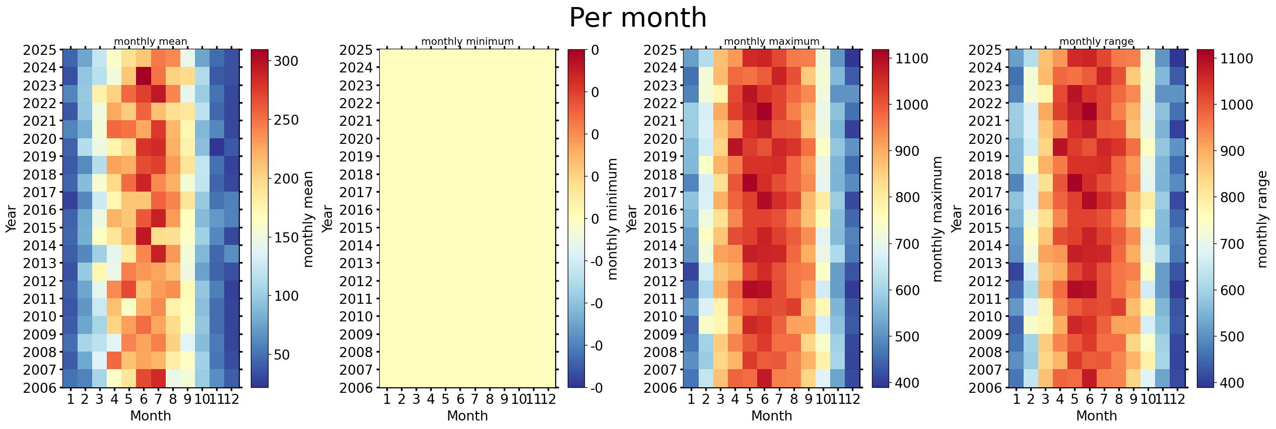
Heatmap plots

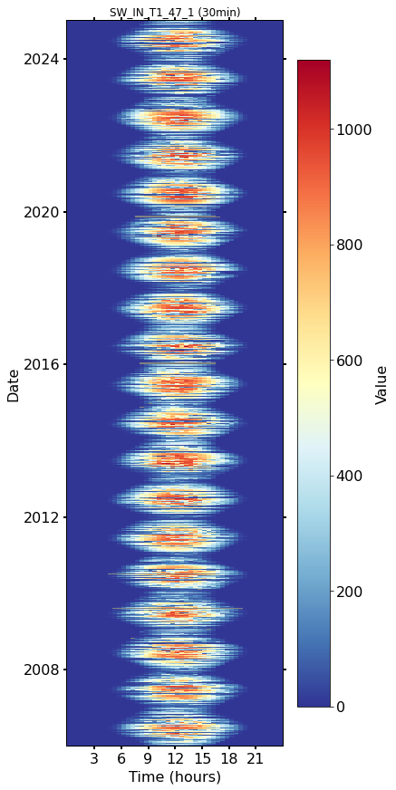
Half-hourly

fig, axs = plt.subplots(ncols=1, figsize=(6, 12), dpi=72, layout="constrained")
dv.heatmapdatetime(series=series, ax=axs, cb_digits_after_comma=0).plot()

Monthly

fig, axs = plt.subplots(ncols=4, figsize=(21, 7), dpi=120, layout="constrained")
fig.suptitle(f'Per month', fontsize=32)
dv.heatmapyearmonth(series_monthly=series.resample('M').mean(), title="monthly mean", ax=axs[0], cb_digits_after_comma=0, zlabel="monthly mean").plot()
dv.heatmapyearmonth(series_monthly=series.resample('M').min(), title="monthly minimum", ax=axs[1], cb_digits_after_comma=0, zlabel="monthly minimum").plot()
dv.heatmapyearmonth(series_monthly=series.resample('M').max(), title="monthly maximum", ax=axs[2], cb_digits_after_comma=0, zlabel="monthly maximum").plot()
_range = series.resample('M').max().sub(series.resample('M').min())
dv.heatmapyearmonth(series_monthly=_range, title="monthly range", ax=axs[3], cb_digits_after_comma=0, zlabel="monthly range").plot()

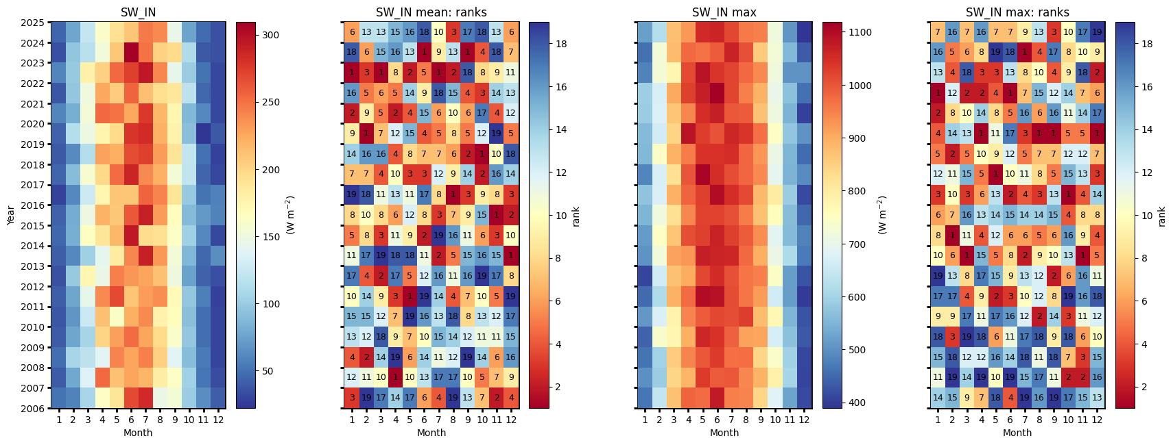
Monthly ranks

# Figure
fig = plt.figure(facecolor='white', figsize=(17, 6))

# Gridspec for layout
gs = gridspec.GridSpec(1, 4)  # rows, cols
gs.update(wspace=0.35, hspace=0.3, left=0.03, right=0.97, top=0.97, bottom=0.03)
ax_mean = fig.add_subplot(gs[0, 0])
ax_mean_ranks = fig.add_subplot(gs[0, 1])
ax_max = fig.add_subplot(gs[0, 2])
ax_max_ranks = fig.add_subplot(gs[0, 3])
params = {'axlabels_fontsize': 10, 'ticks_labelsize': 10, 'cb_labelsize': 10}
dv.heatmapyearmonth_ranks(ax=ax_mean, series=series, agg='mean', ranks=False, zlabel=f"{units}", cmap="RdYlBu_r", show_values=False, **params).plot()

hm_mean_ranks = dv.heatmapyearmonth_ranks(ax=ax_mean_ranks, series=series, agg='mean', **params)
hm_mean_ranks.plot()

dv.heatmapyearmonth_ranks(ax=ax_max, series=series, agg='max', ranks=False, zlabel=f"{units}", cmap="RdYlBu_r", show_values=False, **params).plot()
dv.heatmapyearmonth_ranks(ax=ax_max_ranks, series=series, agg='max', **params).plot()

ax_mean.set_title(f"{var}", color='black')
ax_mean_ranks.set_title(f"{var} mean: ranks", color='black')
ax_max.set_title(f"{var} max", color='black')
ax_max_ranks.set_title(f"{var} max: ranks", color='black')

ax_mean.tick_params(left=True, right=False, top=False, bottom=True,
                    labelleft=True, labelright=False, labeltop=False, labelbottom=True)
ax_mean_ranks.tick_params(left=True, right=False, top=False, bottom=True,
                   labelleft=False, labelright=False, labeltop=False, labelbottom=True)
ax_max.tick_params(left=True, right=False, top=False, bottom=True,
                     labelleft=False, labelright=False, labeltop=False, labelbottom=True)
ax_max_ranks.tick_params(left=True, right=False, top=False, bottom=True,
                     labelleft=False, labelright=False, labeltop=False, labelbottom=True)

ax_mean_ranks.set_ylabel("")
ax_max.set_ylabel("")
ax_max_ranks.set_ylabel("")

fig.show()

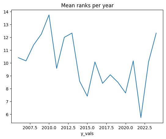
Mean ranks per year

hm_mean_ranks.hm.get_plot_data().mean(axis=1).plot(title="Mean ranks per year");

Ridgeline plots

Yearly

# rp = dv.ridgeline(series=series)
# rp.plot(
#     how='yearly',
#     kd_kwargs=None,  # params from scikit KernelDensity as dict
#     xlim=xlim,  # min/max as list
#     ylim=[0, 0.01],  # min/max as list
#     hspace=-0.8,  # overlap between months
#     xlabel=f"{var} ({units})",
#     fig_width=5,
#     fig_height=9,
#     shade_percentile=0.5,
#     show_mean_line=False,
#     fig_title=f"{var} per year (2005-2024)",
#     fig_dpi=72,
#     showplot=True,
#     ascending=False
# )

Monthly

# rp.plot(
#     how='monthly',
#     kd_kwargs=None,  # params from scikit KernelDensity as dict
#     xlim=xlim,  # min/max as list
#     ylim=[0, 0.01],  # min/max as list
#     hspace=-0.6,  # overlap between months
#     xlabel=f"{var} ({units})",
#     fig_width=4.5,
#     fig_height=8,
#     shade_percentile=0.5,
#     show_mean_line=False,
#     fig_title=f"{var} per month (2005-2024)",
#     fig_dpi=72,
#     showplot=True,
#     ascending=False
# )

Weekly

# rp.plot(
#     how='weekly',
#     kd_kwargs=None,  # params from scikit KernelDensity as dict
#     xlim=xlim,  # min/max as list
#     ylim=[0, 0.15],  # min/max as list
#     hspace=-0.6,  # overlap
#     xlabel=f"{var} ({units})",
#     fig_width=6,
#     fig_height=16,
#     shade_percentile=0.5,
#     show_mean_line=False,
#     fig_title=f"{var} per week (2005-2024)",
#     fig_dpi=72,
#     showplot=True,
#     ascending=False
# )

Single years per month

# uniq_years = series.index.year.unique()
# for uy in uniq_years:
#     series_yr = series.loc[series.index.year == uy].copy()
#     rp = dv.ridgeline(series=series_yr)
#     rp.plot(
#         how='monthly',
#         kd_kwargs=None,  # params from scikit KernelDensity as dict
#         xlim=xlim,  # min/max as list
#         ylim=[0, 0.18],  # min/max as list
#         hspace=-0.6,  # overlap
#         xlabel=f"{var} ({units})",
#         fig_width=6,
#         fig_height=7,
#         shade_percentile=0.5,
#         show_mean_line=False,
#         fig_title=f"{var} per month ({uy})",
#         fig_dpi=72,
#         showplot=True,
#         ascending=False
#     )

Single years per week

# uniq_years = series.index.year.unique()
# for uy in uniq_years:
#     series_yr = series.loc[series.index.year == uy].copy()
#     rp = dv.ridgeline(series=series_yr)
#     rp.plot(
#         how='weekly',
#         kd_kwargs=None,  # params from scikit KernelDensity as dict
#         xlim=xlim,  # min/max as list
#         ylim=[0, 0.3],  # min/max as list
#         hspace=-0.8,  # overlap
#         xlabel=f"{var} ({units})",
#         fig_width=9,
#         fig_height=18,
#         shade_percentile=0.5,
#         show_mean_line=False,
#         fig_title=f"{var} per week ({uy})",
#         fig_dpi=72,
#         showplot=True,
#         ascending=False
#     )

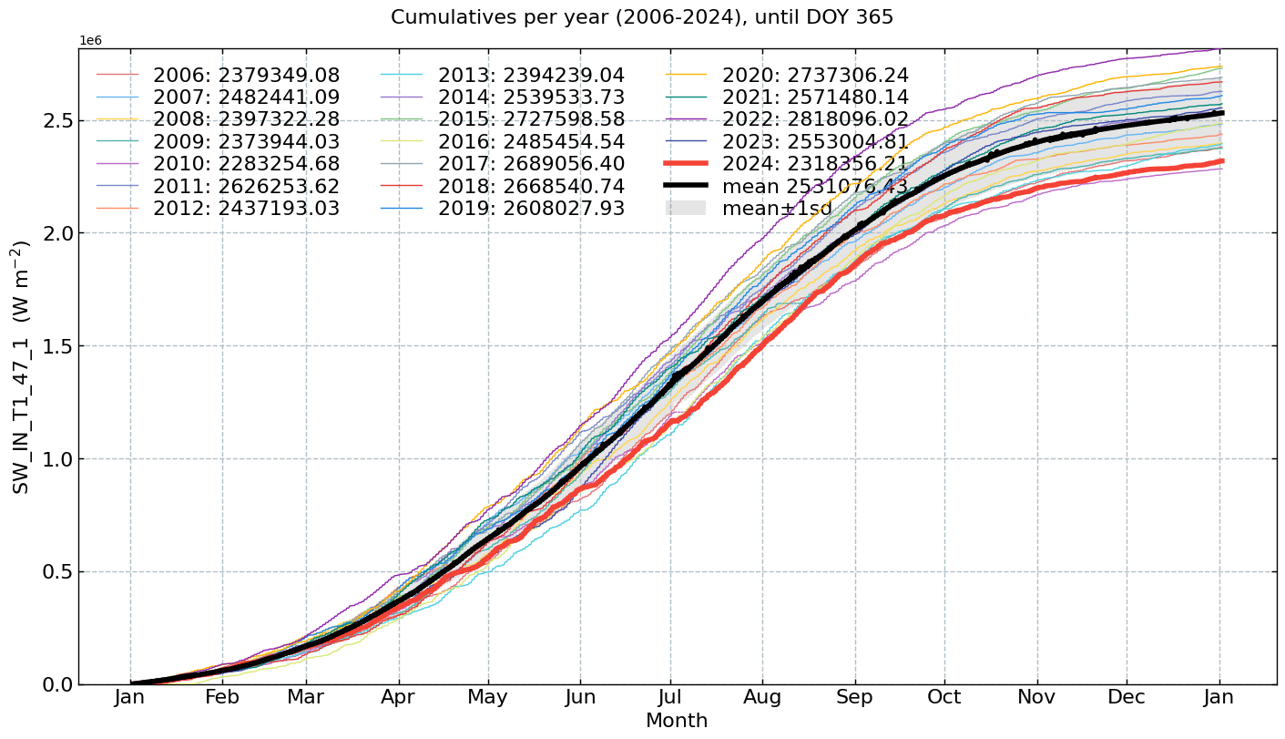
Cumulative plot

CumulativeYear(
    series=series,
    series_units=units,
    start_year=2005,
    end_year=2024,
    show_reference=True,
    excl_years_from_reference=None,
    highlight_year=2024,
    highlight_year_color='#F44336').plot();

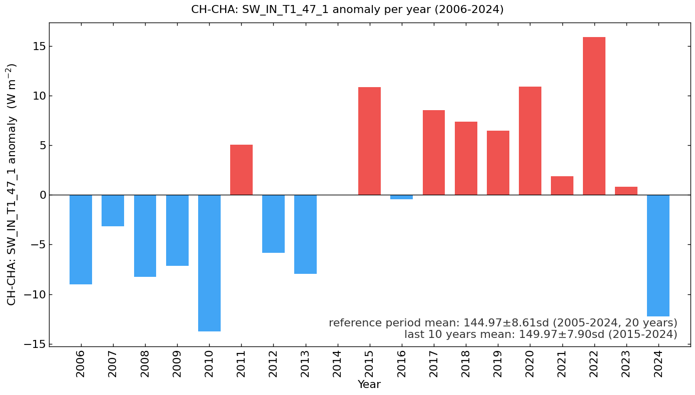
Long-term anomalies

series_yearly_mean = series.resample('YE').mean()
series_yearly_mean.index = series_yearly_mean.index.year
series_label = f"CH-CHA: {varname}"
LongtermAnomaliesYear(series=series_yearly_mean,
                      series_label=series_label,
                      series_units=units,
                      reference_start_year=2005,
                      reference_end_year=2024).plot()

End of notebook

dt_string = datetime.now().strftime("%Y-%m-%d %H:%M:%S")
print(f"Finished. {dt_string}")

Finished. 2025-06-11 22:13:59