Meteo: Air temperature (TA) (2005-2024)

Author: Lukas Hörtnagl (holukas@ethz.ch)

Variable

varname = 'TA_T1_47_1_gfXG'
var = "TA"  # Name shown in plots
units = "°C"

Imports

import importlib.metadata
import warnings
from datetime import datetime
from pathlib import Path
import pandas as pd
import matplotlib.pyplot as plt
import matplotlib.gridspec as gridspec

import diive as dv
from diive.core.io.files import save_parquet, load_parquet
from diive.core.plotting.cumulative import CumulativeYear
from diive.core.plotting.bar import LongtermAnomaliesYear

warnings.filterwarnings(action='ignore', category=FutureWarning)
warnings.filterwarnings(action='ignore', category=UserWarning)
version_diive = importlib.metadata.version("diive")
print(f"diive version: v{version_diive}")

diive version: v0.87.0

Load data

SOURCEDIR = r"../10_METEO"
FILENAME = r"12.3_METEO_GAPFILLED_2004-2024.parquet"
FILEPATH = Path(SOURCEDIR) / FILENAME
df = load_parquet(filepath=FILEPATH)
keeplocs = (df.index.year >= 2005) & (df.index.year <= 2024)
df = df[keeplocs].copy()
df

Loaded .parquet file ..\10_METEO\12.3_METEO_GAPFILLED_2004-2024.parquet (0.024 seconds).
    --> Detected time resolution of <30 * Minutes> / 30min 

	LW_IN_T1_47_1	PA_T1_47_1	PPFD_IN_T1_47_1	RH_T1_47_1	SW_IN_T1_47_1	TA_T1_47_1	SW_IN_T1_47_1_gfXG	TA_T1_47_1_gfXG	PPFD_IN_T1_47_1_gfXG
TIMESTAMP_MIDDLE
2005-01-01 00:15:00	NaN	NaN	0.0	96.203705	0.0	-2.160000	0.0	-2.160000	0.0
2005-01-01 00:45:00	NaN	NaN	0.0	98.003701	0.0	-2.010000	0.0	-2.010000	0.0
2005-01-01 01:15:00	NaN	NaN	0.0	98.203705	0.0	-1.791000	0.0	-1.791000	0.0
2005-01-01 01:45:00	NaN	NaN	0.0	98.203705	0.0	-1.539000	0.0	-1.539000	0.0
2005-01-01 02:15:00	NaN	NaN	0.0	98.203705	0.0	-1.338000	0.0	-1.338000	0.0
...	...	...	...	...	...	...	...	...	...
2024-12-31 21:45:00	232.595527	94.211806	0.0	87.254008	0.0	-0.504794	0.0	-0.504794	0.0
2024-12-31 22:15:00	232.609777	94.189013	0.0	87.430236	0.0	-0.296828	0.0	-0.296828	0.0
2024-12-31 22:45:00	232.345020	94.169525	0.0	89.787920	0.0	-0.392922	0.0	-0.392922	0.0
2024-12-31 23:15:00	234.211100	94.168413	0.0	81.809355	0.0	0.792661	0.0	0.792661	0.0
2024-12-31 23:45:00	231.760533	94.170793	0.0	88.311314	0.0	-0.422600	0.0	-0.422600	0.0

350640 rows × 9 columns

series = df[varname].copy()
series

TIMESTAMP_MIDDLE
2005-01-01 00:15:00   -2.160000
2005-01-01 00:45:00   -2.010000
2005-01-01 01:15:00   -1.791000
2005-01-01 01:45:00   -1.539000
2005-01-01 02:15:00   -1.338000
                         ...   
2024-12-31 21:45:00   -0.504794
2024-12-31 22:15:00   -0.296828
2024-12-31 22:45:00   -0.392922
2024-12-31 23:15:00    0.792661
2024-12-31 23:45:00   -0.422600
Freq: 30min, Name: TA_T1_47_1_gfXG, Length: 350640, dtype: float64

xlabel = f"{var} ({units})"
xlim = [series.min(), series.max()]

Stats

Overall mean

_yearly_avg = series.resample('YE').mean()
_overall_mean = _yearly_avg.mean()
_overall_sd = _yearly_avg.std()
print(f"Overall mean: {_overall_mean} +/- {_overall_sd}")

Overall mean: 8.9549543810582 +/- 1.3482554138577252

Yearly means

ym = series.resample('YE').mean()
ym

TIMESTAMP_MIDDLE
2005-12-31     7.429217
2006-12-31     7.960293
2007-12-31     8.109144
2008-12-31     7.588395
2009-12-31     7.948623
2010-12-31     6.803609
2011-12-31     8.786543
2012-12-31     7.823660
2013-12-31     7.106809
2014-12-31     8.703434
2015-12-31     8.736166
2016-12-31     9.558060
2017-12-31     9.759068
2018-12-31    10.702271
2019-12-31    10.291331
2020-12-31    10.504883
2021-12-31     9.056597
2022-12-31    11.120893
2023-12-31    10.765006
2024-12-31    10.345086
Freq: YE-DEC, Name: TA_T1_47_1_gfXG, dtype: float64

ym.sort_values(ascending=False)

TIMESTAMP_MIDDLE
2022-12-31    11.120893
2023-12-31    10.765006
2018-12-31    10.702271
2020-12-31    10.504883
2024-12-31    10.345086
2019-12-31    10.291331
2017-12-31     9.759068
2016-12-31     9.558060
2021-12-31     9.056597
2011-12-31     8.786543
2015-12-31     8.736166
2014-12-31     8.703434
2007-12-31     8.109144
2006-12-31     7.960293
2009-12-31     7.948623
2012-12-31     7.823660
2008-12-31     7.588395
2005-12-31     7.429217
2013-12-31     7.106809
2010-12-31     6.803609
Name: TA_T1_47_1_gfXG, dtype: float64

Monthly averages

seriesdf = pd.DataFrame(series)
seriesdf['MONTH'] = seriesdf.index.month
seriesdf['YEAR'] = seriesdf.index.year
monthly_avg = seriesdf.groupby(['YEAR', 'MONTH'])[varname].mean().unstack()
monthly_avg

MONTH	1	2	3	4	5	6	7	8	9	10	11	12
YEAR
2005	-1.798928	-3.298467	3.613463	7.327779	11.914164	16.726858	16.591920	14.460255	13.816814	9.833265	2.185859	-2.926974
2006	-4.194532	-2.299361	0.443276	6.594224	11.012580	16.028185	21.033602	12.454961	15.517356	11.289903	6.052256	0.996613
2007	1.831280	2.950667	3.866424	12.747250	12.409842	14.977545	15.420882	15.238803	11.221396	7.458473	0.789296	-1.865884
2008	1.498027	2.287706	1.880655	5.617952	13.469550	15.097302	16.143572	15.790118	10.281068	7.840179	2.565744	-1.649615
2009	-3.974498	-1.601780	1.854548	10.023973	13.505490	14.196945	16.561570	18.342514	13.991227	7.741110	5.356225	-1.158283
2010	-4.242044	-1.379788	2.465842	8.187206	9.017224	15.094503	18.229335	15.085477	11.608217	7.024903	2.883811	-2.782696
2011	-0.923986	1.041491	4.759064	11.375054	13.705819	14.686286	14.439601	17.685672	14.965174	7.767536	4.262686	1.251798
2012	-0.385405	-5.501142	7.017484	6.471191	12.224344	15.266384	15.645665	17.539556	12.566301	8.192080	4.585683	-0.352892
2013	-1.854887	-3.664084	0.365234	6.492476	8.224684	13.956154	19.142624	16.977072	12.762685	9.517883	1.539382	0.984121
2014	1.166215	1.926494	5.892282	8.911640	10.221405	16.247756	15.719818	14.138015	13.661444	10.812444	4.943577	0.433012
2015	-0.440557	-2.097140	4.544967	8.231290	11.547104	15.871719	20.327214	18.712603	11.211259	6.926023	5.430528	3.707700
2016	0.890098	2.837591	4.041670	8.268441	12.593452	15.919292	19.398752	19.365958	17.255841	8.328448	4.340064	1.267124
2017	-3.730232	3.588457	8.196496	8.314217	14.401430	19.210224	18.936156	19.645432	12.807543	11.445372	3.735386	0.123475
2018	3.651935	-2.672235	3.066301	13.204716	14.698813	17.746751	20.973403	20.693080	16.709867	11.710273	5.212166	2.462536
2019	-0.989104	4.319631	6.510257	8.886606	10.056998	19.499712	20.484599	19.035565	14.931494	11.209238	6.008235	3.228077
2020	2.249733	5.005212	5.196607	12.761152	13.198056	15.644990	19.662248	19.723812	16.071764	8.949485	5.625622	1.875873
2021	-0.506040	4.147604	5.117351	7.316763	9.631604	18.450182	17.368270	16.548159	16.255653	9.689530	2.887954	1.577205
2022	0.922858	3.473913	7.477323	8.347545	15.615285	19.285291	21.095167	20.425183	13.606485	14.086912	6.538461	1.942527
2023	1.527202	3.165265	6.046677	6.899131	13.109495	19.705106	19.507541	19.522261	18.653598	13.107932	4.396678	3.016453
2024	1.331627	5.929059	7.444291	9.292731	12.905508	16.810613	19.461952	20.934985	13.727278	11.096496	4.329863	0.681400

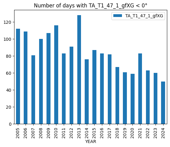
Number of days below 0°C

plotdf = df[[varname]].copy()
plotdf = plotdf.resample('D').min()
belowzero = plotdf.loc[plotdf[varname] < 0].copy()
belowzero = belowzero.groupby(belowzero.index.year).count()
belowzero["YEAR"] = belowzero.index
belowzero
belowzero.plot.bar(x="YEAR", y=varname, title=f"Number of days with {varname} < 0°");
display(belowzero)
print(f"Average per year: {belowzero[varname].mean()} +/- {belowzero[varname].std():.2f} SD")

	TA_T1_47_1_gfXG	YEAR
TIMESTAMP_MIDDLE
2005	112	2005
2006	109	2006
2007	81	2007
2008	100	2008
2009	107	2009
2010	116	2010
2011	83	2011
2012	91	2012
2013	128	2013
2014	76	2014
2015	87	2015
2016	83	2016
2017	82	2017
2018	67	2018
2019	61	2019
2020	59	2020
2021	83	2021
2022	63	2022
2023	60	2023
2024	50	2024

Average per year: 84.9 +/- 21.63 SD

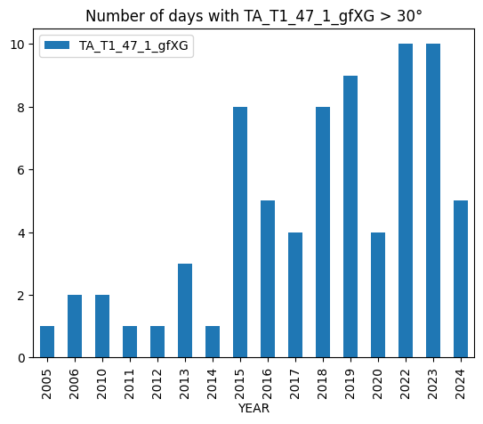
Number of days above 30°C

plotdf = df[[varname]].copy()
plotdf = plotdf.resample('D').max()
above = plotdf.loc[plotdf[varname] > 30].copy()
above = above.groupby(above.index.year).count()
above["YEAR"] = above.index
above.plot.bar(x="YEAR", y=varname, title=f"Number of days with {varname} > 30°");
display(above)
print(f"Average per year: {above[varname].mean()} +/- {above[varname].std():.2f} SD")

	TA_T1_47_1_gfXG	YEAR
TIMESTAMP_MIDDLE
2005	1	2005
2006	2	2006
2010	2	2010
2011	1	2011
2012	1	2012
2013	3	2013
2014	1	2014
2015	8	2015
2016	5	2016
2017	4	2017
2018	8	2018
2019	9	2019
2020	4	2020
2022	10	2022
2023	10	2023
2024	5	2024

Average per year: 4.625 +/- 3.36 SD

Heatmap plots

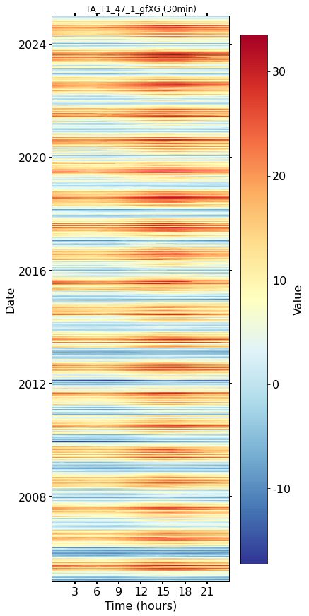
Half-hourly

fig, axs = plt.subplots(ncols=1, figsize=(6, 12), dpi=72, layout="constrained")
dv.heatmapdatetime(series=series, ax=axs, cb_digits_after_comma=0).plot()

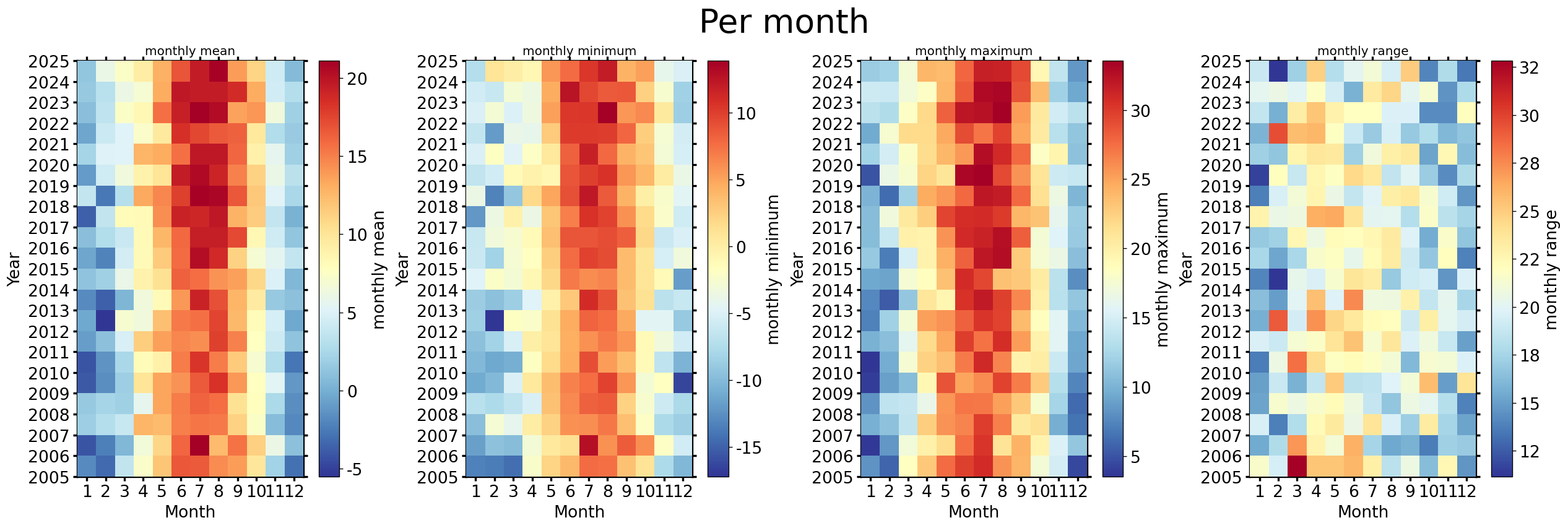
Monthly

fig, axs = plt.subplots(ncols=4, figsize=(21, 7), dpi=120, layout="constrained")
fig.suptitle(f'Per month', fontsize=32)
dv.heatmapyearmonth(series_monthly=series.resample('M').mean(), title="monthly mean", ax=axs[0], cb_digits_after_comma=0, zlabel="monthly mean").plot()
dv.heatmapyearmonth(series_monthly=series.resample('M').min(), title="monthly minimum", ax=axs[1], cb_digits_after_comma=0, zlabel="monthly minimum").plot()
dv.heatmapyearmonth(series_monthly=series.resample('M').max(), title="monthly maximum", ax=axs[2], cb_digits_after_comma=0, zlabel="monthly maximum").plot()
_range = series.resample('M').max().sub(series.resample('M').min())
dv.heatmapyearmonth(series_monthly=_range, title="monthly range", ax=axs[3], cb_digits_after_comma=0, zlabel="monthly range").plot()

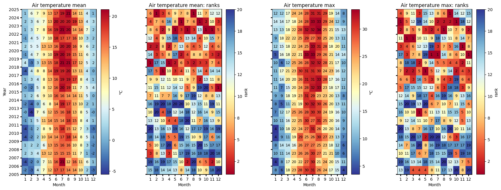
Monthly ranks

# Figure
fig = plt.figure(facecolor='white', figsize=(17, 6))

# Gridspec for layout
gs = gridspec.GridSpec(1, 4)  # rows, cols
gs.update(wspace=0.35, hspace=0.3, left=0.03, right=0.97, top=0.97, bottom=0.03)
ax_mean = fig.add_subplot(gs[0, 0])
ax_mean_ranks = fig.add_subplot(gs[0, 1])
ax_max = fig.add_subplot(gs[0, 2])
ax_max_ranks = fig.add_subplot(gs[0, 3])
params = {'axlabels_fontsize': 10, 'ticks_labelsize': 10, 'cb_labelsize': 10}
dv.heatmapyearmonth_ranks(ax=ax_mean, series=series, agg='mean', ranks=False, zlabel="°C", cmap="RdYlBu_r", show_values=True, **params).plot()

hm_mean_ranks = dv.heatmapyearmonth_ranks(ax=ax_mean_ranks, series=series, agg='mean', show_values=True, **params)
hm_mean_ranks.plot()

dv.heatmapyearmonth_ranks(ax=ax_max, series=series, agg='max', ranks=False, zlabel="°C", cmap="RdYlBu_r", show_values=True, **params).plot()
dv.heatmapyearmonth_ranks(ax=ax_max_ranks, series=series, agg='max', show_values=True, **params).plot()

ax_mean.set_title("Air temperature mean", color='black')
ax_mean_ranks.set_title("Air temperature mean: ranks", color='black')
ax_max.set_title("Air temperature max", color='black')
ax_max_ranks.set_title("Air temperature max: ranks", color='black')

ax_mean.tick_params(left=True, right=False, top=False, bottom=True,
                    labelleft=True, labelright=False, labeltop=False, labelbottom=True)
ax_mean_ranks.tick_params(left=True, right=False, top=False, bottom=True,
                   labelleft=False, labelright=False, labeltop=False, labelbottom=True)
ax_max.tick_params(left=True, right=False, top=False, bottom=True,
                     labelleft=False, labelright=False, labeltop=False, labelbottom=True)
ax_max_ranks.tick_params(left=True, right=False, top=False, bottom=True,
                     labelleft=False, labelright=False, labeltop=False, labelbottom=True)

ax_mean_ranks.set_ylabel("")
ax_max.set_ylabel("")
ax_max_ranks.set_ylabel("")

fig.show()

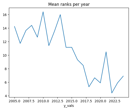
Mean ranks per year

hm_mean_ranks.hm.get_plot_data().mean(axis=1).plot(title="Mean ranks per year");

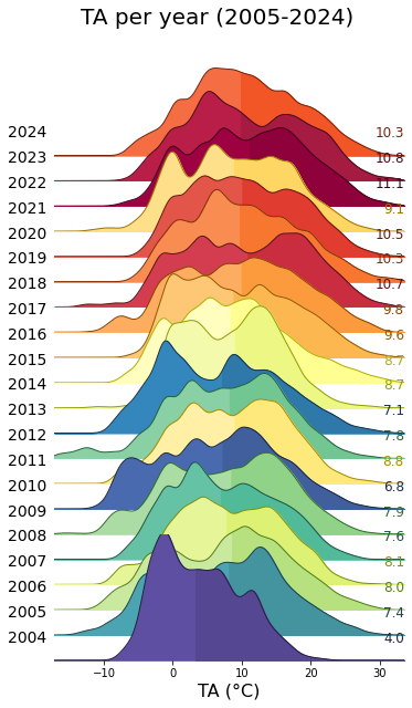
Ridgeline plots

Yearly

rp = dv.ridgeline(series=series)
rp.plot(
    how='yearly',
    kd_kwargs=None,  # params from scikit KernelDensity as dict
    xlim=xlim,  # min/max as list
    ylim=[0, 0.07],  # min/max as list
    hspace=-0.8,  # overlap between months
    xlabel=f"{var} ({units})",
    fig_width=5,
    fig_height=9,
    shade_percentile=0.5,
    show_mean_line=False,
    fig_title=f"{var} per year",
    fig_dpi=72,
    showplot=True,
    ascending=False
)

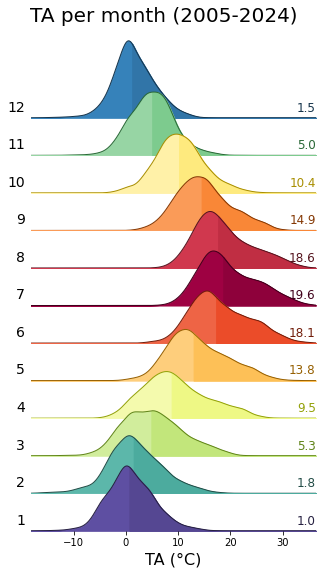
Monthly

rp.plot(
    how='monthly',
    kd_kwargs=None,  # params from scikit KernelDensity as dict
    xlim=xlim,  # min/max as list
    ylim=[0, 0.14],  # min/max as list
    hspace=-0.6,  # overlap between months
    xlabel=f"{var} ({units})",
    fig_width=4.5,
    fig_height=8,
    shade_percentile=0.5,
    show_mean_line=False,
    fig_title=f"{var} per month (2005-2024)",
    fig_dpi=72,
    showplot=True,
    ascending=False
)

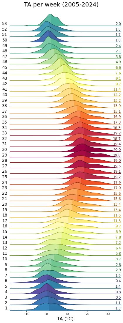
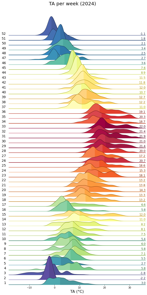
Weekly

rp.plot(
    how='weekly',
    kd_kwargs=None,  # params from scikit KernelDensity as dict
    xlim=xlim,  # min/max as list
    ylim=[0, 0.15],  # min/max as list
    hspace=-0.6,  # overlap
    xlabel=f"{var} ({units})",
    fig_width=6,
    fig_height=16,
    shade_percentile=0.5,
    show_mean_line=False,
    fig_title=f"{var} per week (2005-2024)",
    fig_dpi=72,
    showplot=True,
    ascending=False
)

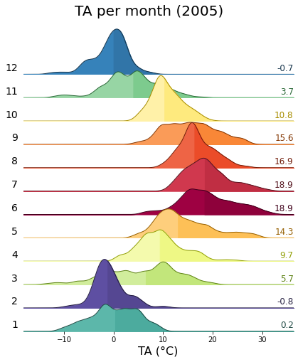
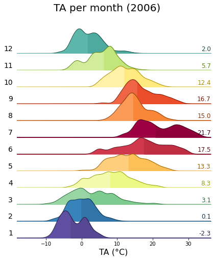
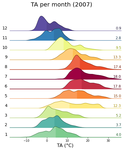
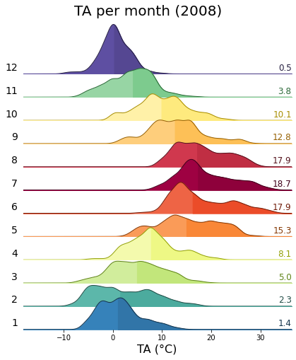
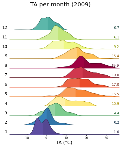
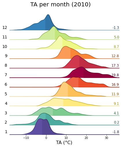
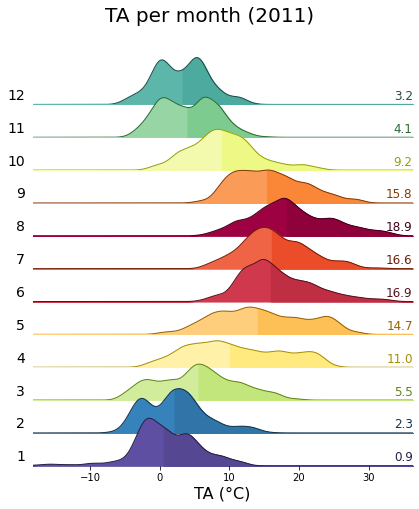
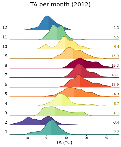
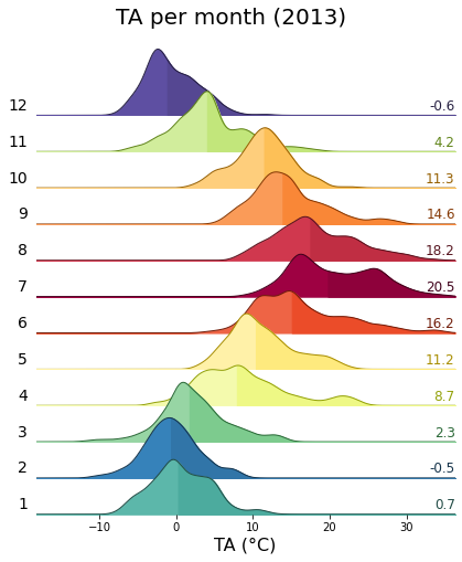
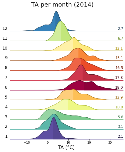
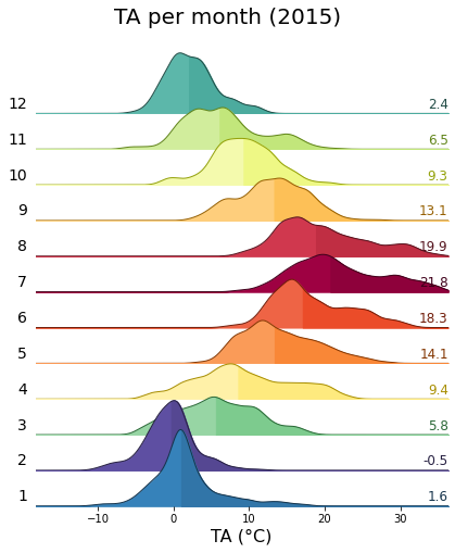
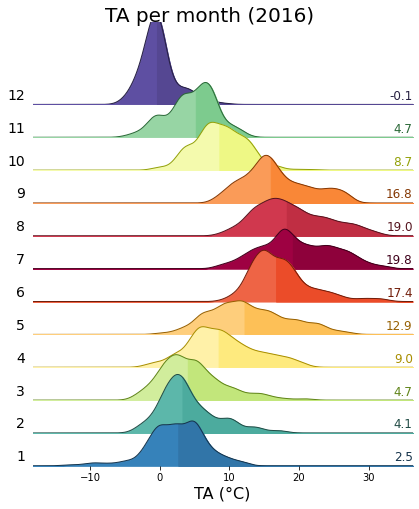
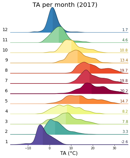
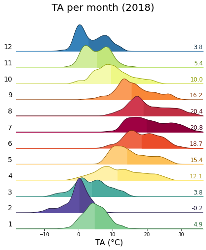
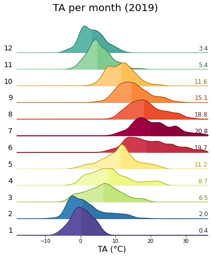
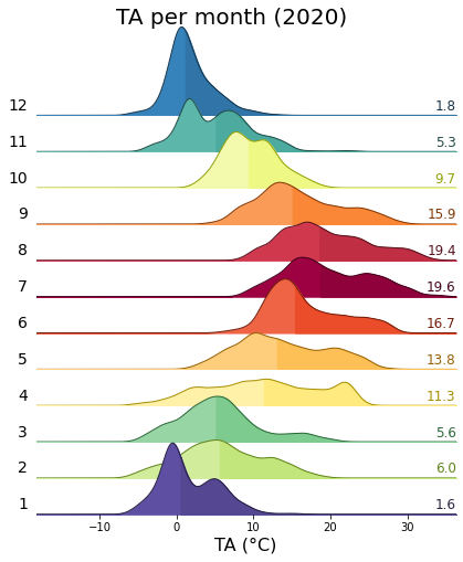
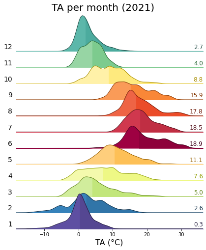
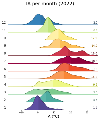
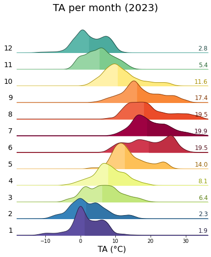
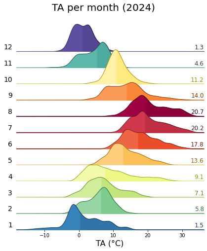
Single years per month

uniq_years = series.index.year.unique()
for uy in uniq_years:
    series_yr = series.loc[series.index.year == uy].copy()
    rp = dv.ridgeline(series=series_yr)
    rp.plot(
        how='monthly',
        kd_kwargs=None,  # params from scikit KernelDensity as dict
        xlim=xlim,  # min/max as list
        ylim=[0, 0.18],  # min/max as list
        hspace=-0.6,  # overlap
        xlabel=f"{var} ({units})",
        fig_width=6,
        fig_height=7,
        shade_percentile=0.5,
        show_mean_line=False,
        fig_title=f"{var} per month ({uy})",
        fig_dpi=72,
        showplot=True,
        ascending=False
    )

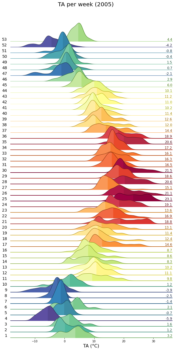
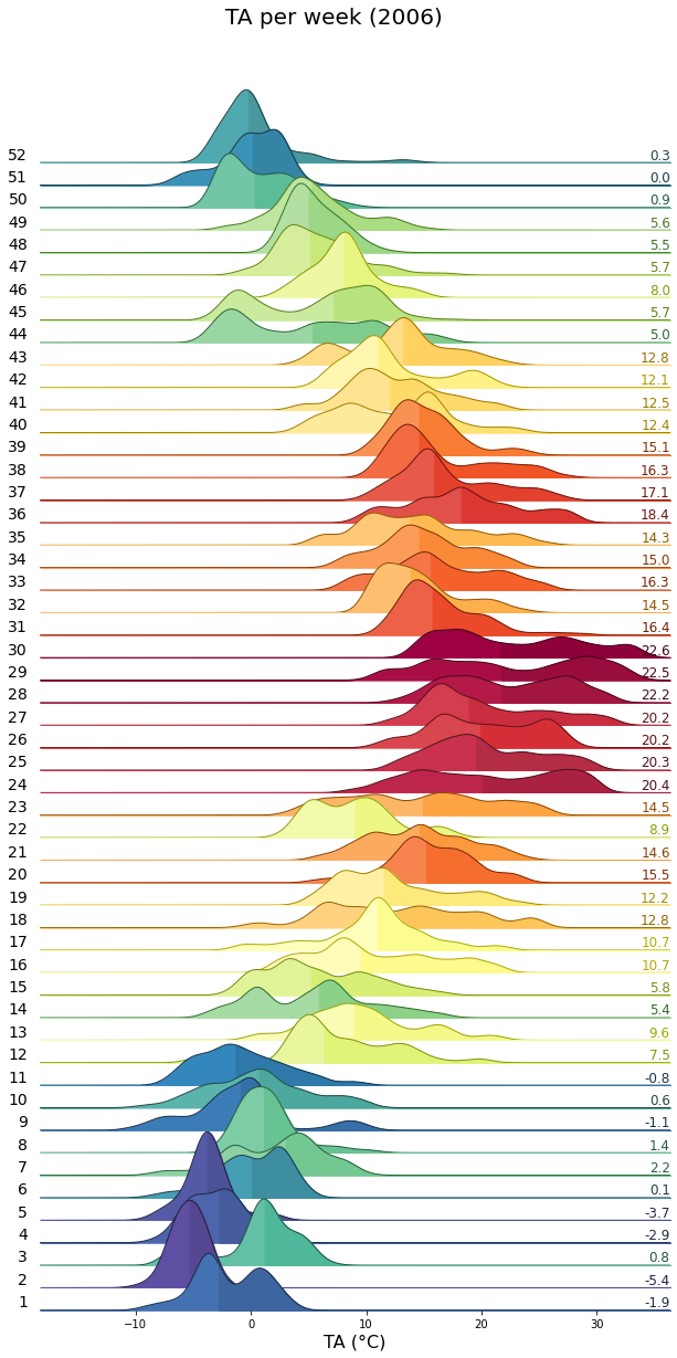
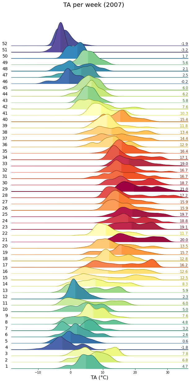
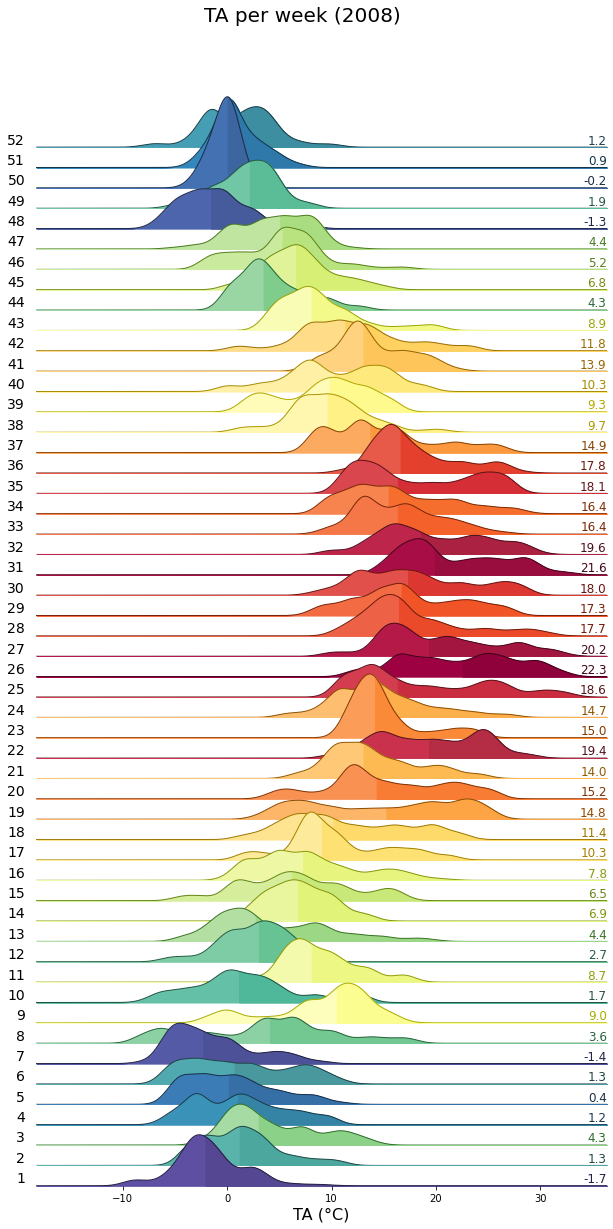
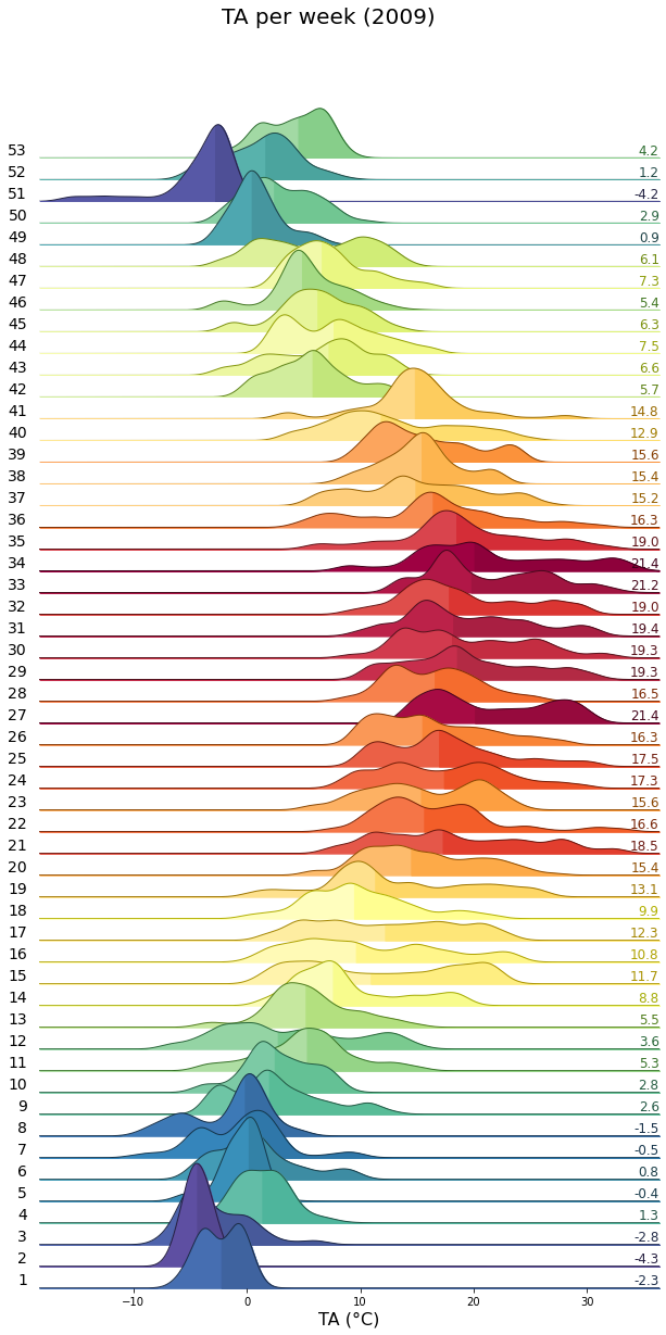
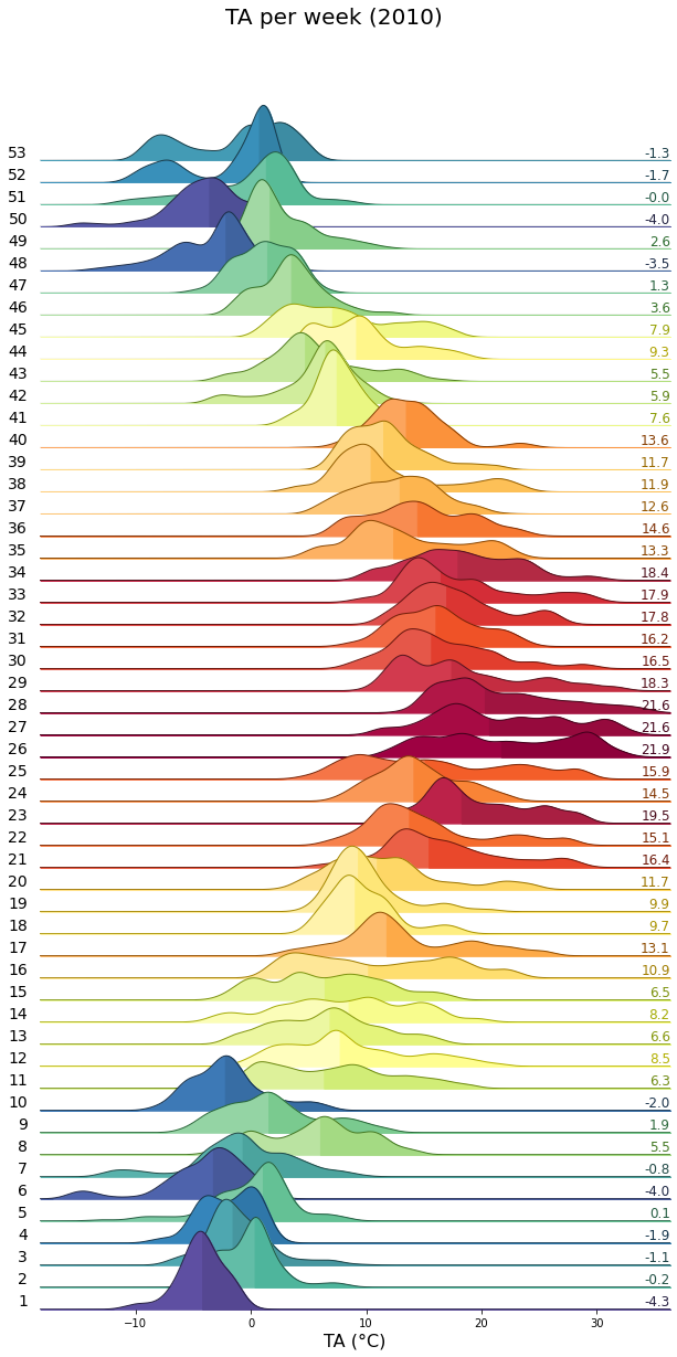
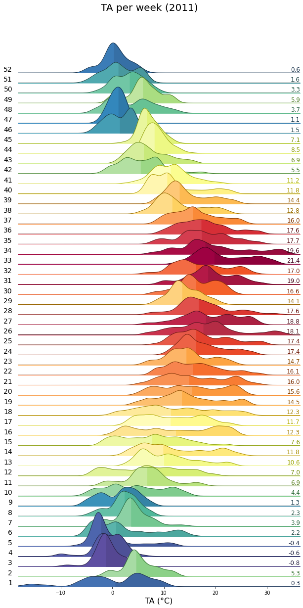
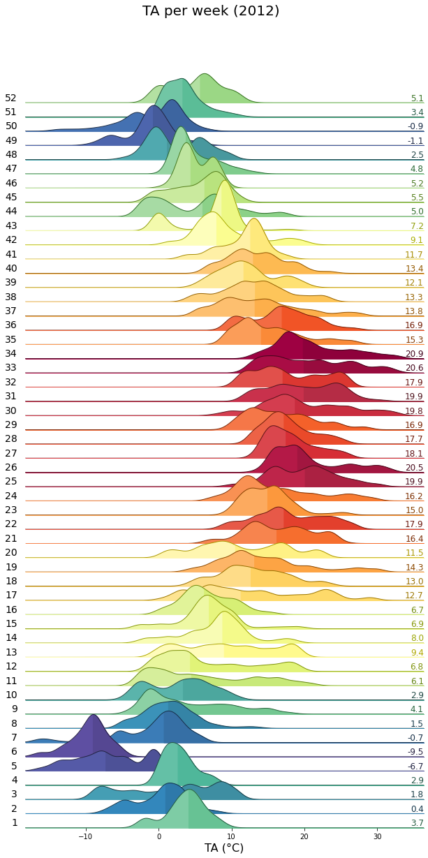
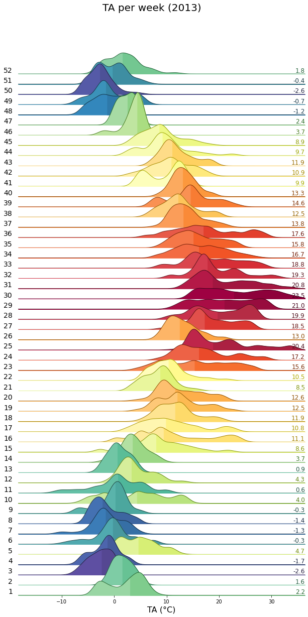
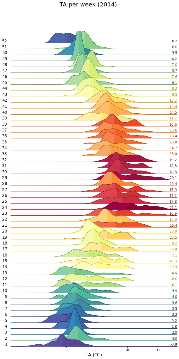
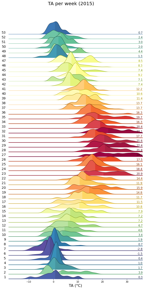
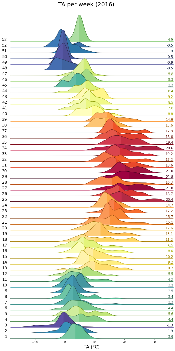
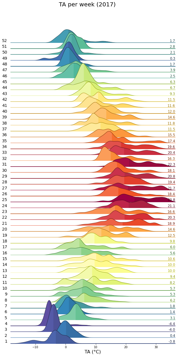
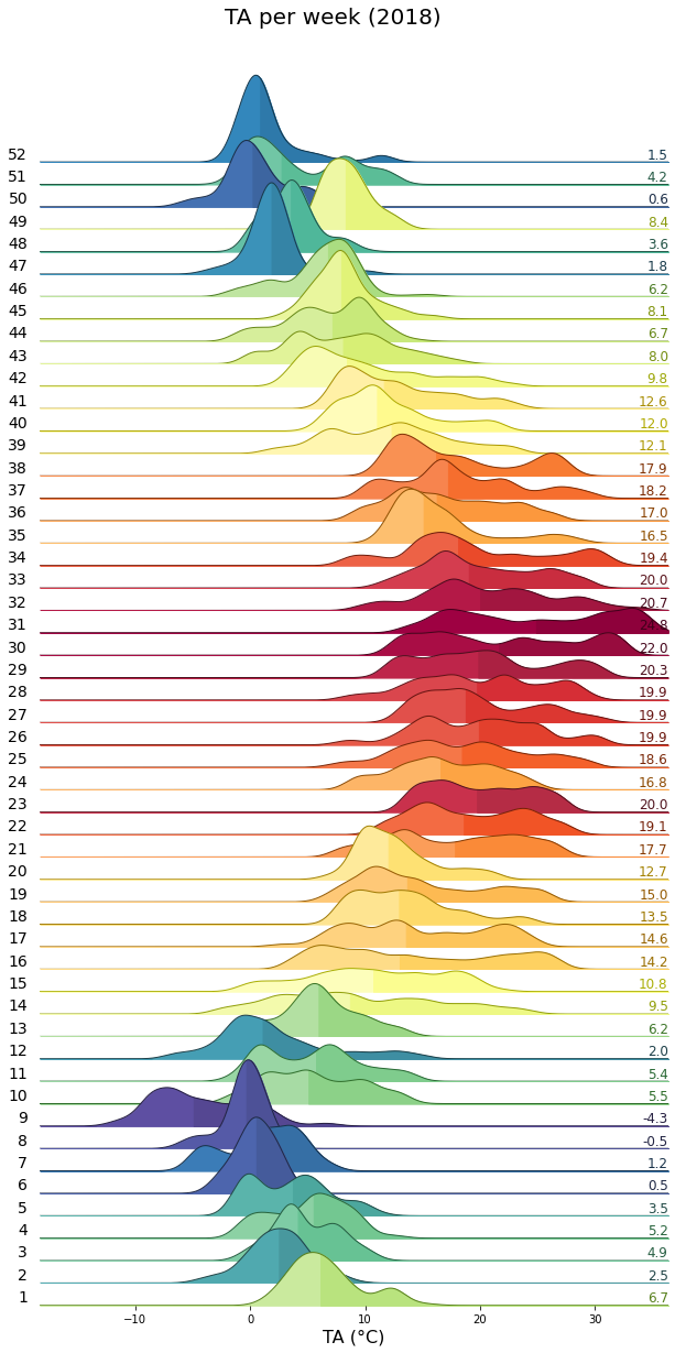
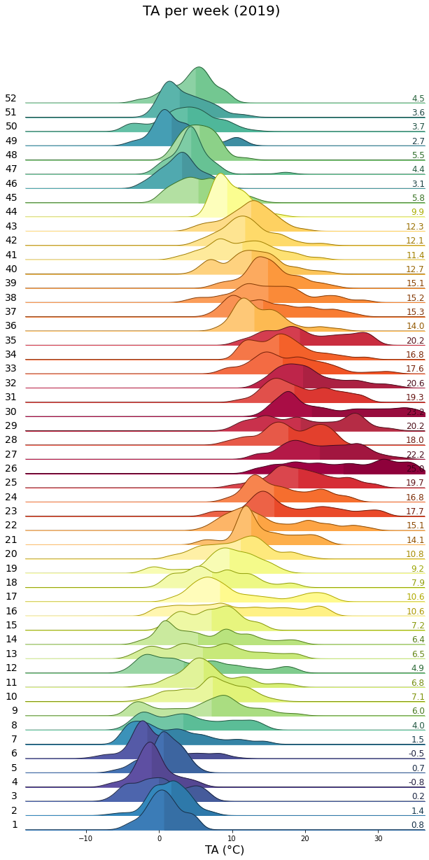
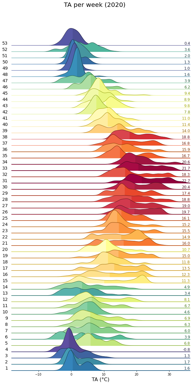
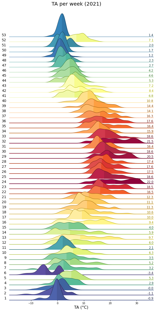
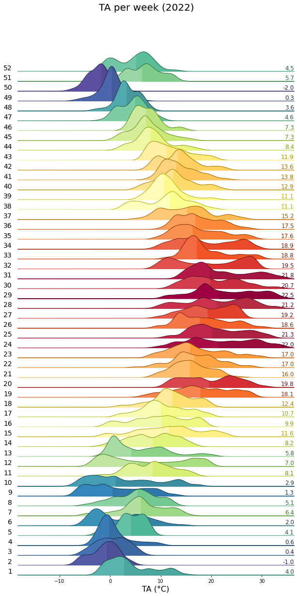
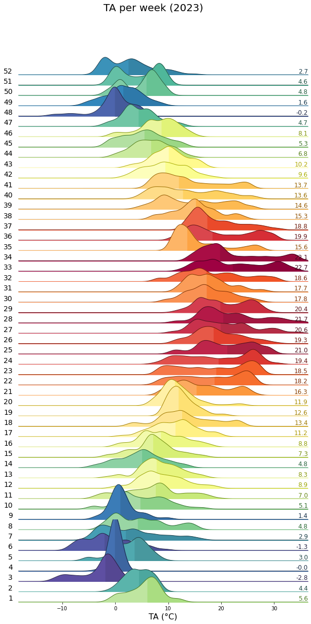
Single years per week

uniq_years = series.index.year.unique()
for uy in uniq_years:
    series_yr = series.loc[series.index.year == uy].copy()
    rp = dv.ridgeline(series=series_yr)
    rp.plot(
        how='weekly',
        kd_kwargs=None,  # params from scikit KernelDensity as dict
        xlim=xlim,  # min/max as list
        ylim=[0, 0.3],  # min/max as list
        hspace=-0.8,  # overlap
        xlabel=f"{var} ({units})",
        fig_width=9,
        fig_height=18,
        shade_percentile=0.5,
        show_mean_line=False,
        fig_title=f"{var} per week ({uy})",
        fig_dpi=72,
        showplot=True,
        ascending=False
    )

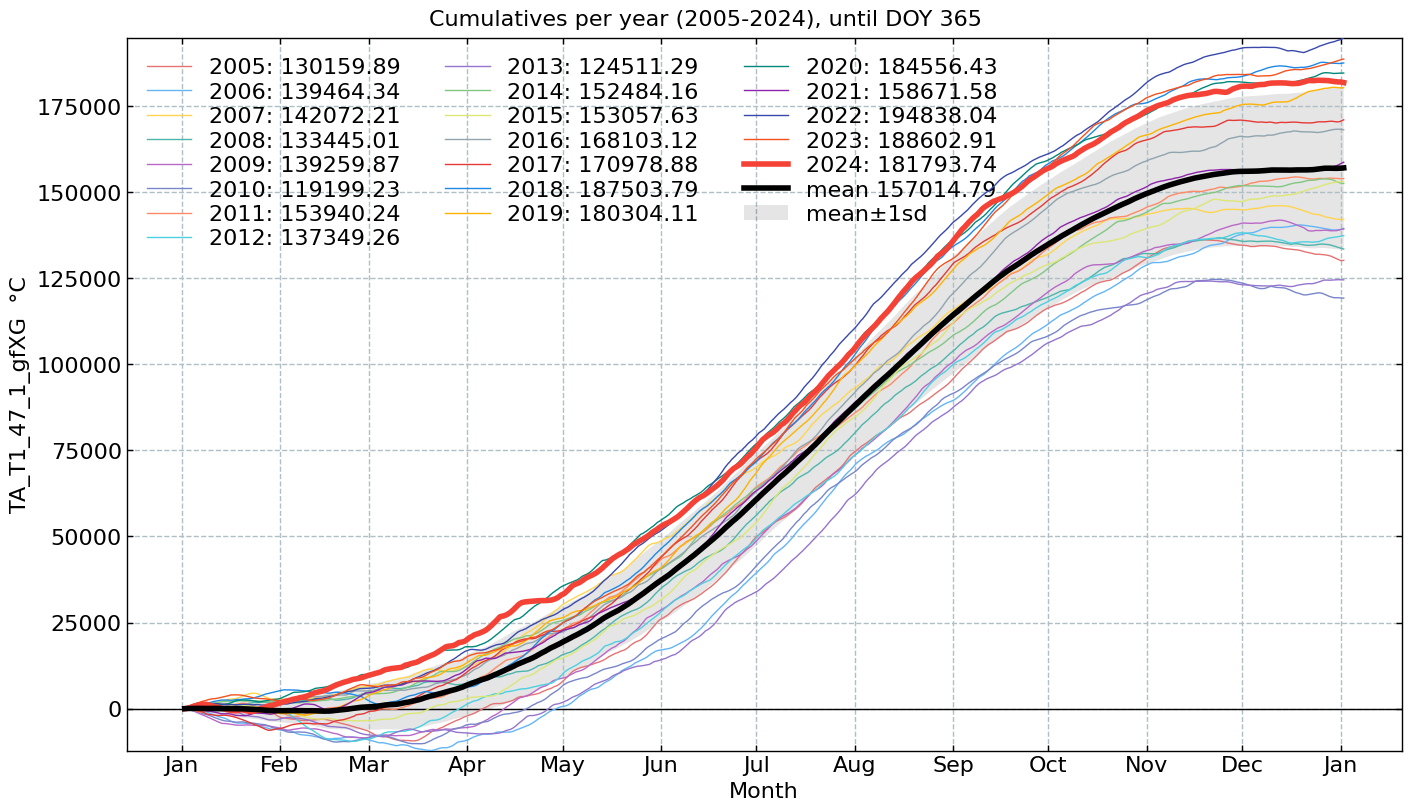
Cumulative plot

CumulativeYear(
    series=series,
    series_units=units,
    start_year=2005,
    end_year=2024,
    show_reference=True,
    excl_years_from_reference=None,
    highlight_year=2024,
    highlight_year_color='#F44336').plot();

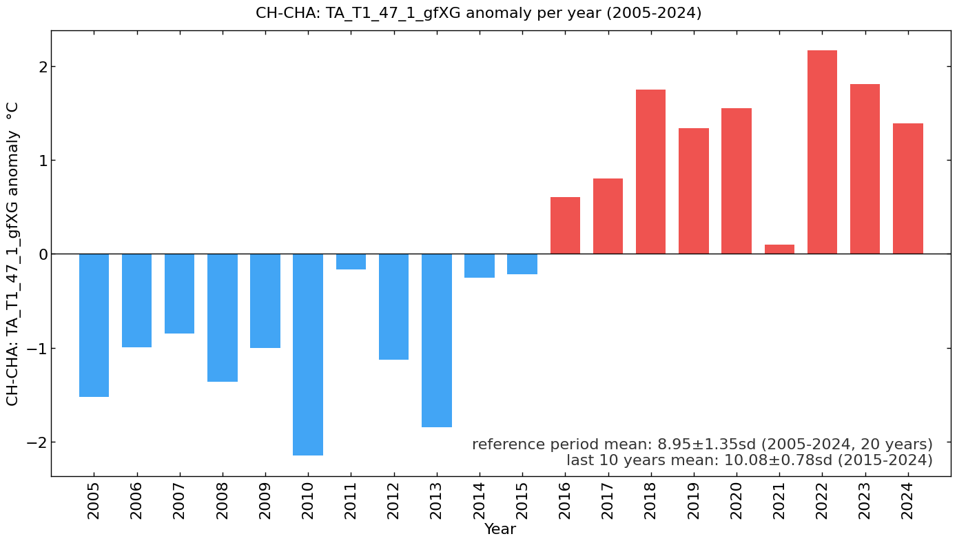
Long-term anomalies

series_yearly_mean = series.resample('YE').mean()
series_yearly_mean.index = series_yearly_mean.index.year
series_label = f"CH-CHA: {varname}"
LongtermAnomaliesYear(series=series_yearly_mean,
                      series_label=series_label,
                      series_units=units,
                      reference_start_year=2005,
                      reference_end_year=2024).plot()

End of notebook

dt_string = datetime.now().strftime("%Y-%m-%d %H:%M:%S")
print(f"Finished. {dt_string}")

Finished. 2025-06-11 16:45:15