Meteo: Air temperature (VPD) (2005-2024)

Author: Lukas Hörtnagl (holukas@ethz.ch)

Variable

varname = 'VPD_T1_47_1'
var = "VPD"  # Name shown in plots
units = "kPa"

Imports

import importlib.metadata
import warnings
from datetime import datetime
from pathlib import Path
import pandas as pd
import matplotlib.pyplot as plt
import matplotlib.gridspec as gridspec

import diive as dv
from diive.core.io.files import save_parquet, load_parquet
from diive.core.plotting.cumulative import CumulativeYear
from diive.core.plotting.bar import LongtermAnomaliesYear

warnings.filterwarnings(action='ignore', category=FutureWarning)
warnings.filterwarnings(action='ignore', category=UserWarning)
version_diive = importlib.metadata.version("diive")
print(f"diive version: v{version_diive}")

diive version: v0.87.1

Load data

SOURCEDIR = r"../10_METEO"
FILENAME = r"12.5_METEO7_GAPFILLED_2004-2024.parquet"
FILEPATH = Path(SOURCEDIR) / FILENAME
df = load_parquet(filepath=FILEPATH)
keeplocs = (df.index.year >= 2005) & (df.index.year <= 2024)
df = df[keeplocs].copy()
df

Loaded .parquet file ..\10_METEO\12.5_METEO7_GAPFILLED_2004-2024.parquet (0.049 seconds).
    --> Detected time resolution of <30 * Minutes> / 30min 

	LW_IN_T1_47_1	PA_T1_47_1	PPFD_IN_T1_47_1	RH_T1_47_1	SW_IN_T1_47_1	TA_T1_47_1	SW_IN_T1_47_1_gfXG	TA_T1_47_1_gfXG	PPFD_IN_T1_47_1_gfXG	VPD_T1_47_1	VPD_T1_47_1_gfXG	FLAG_VPD_T1_47_1_gfXG_ISFILLED
TIMESTAMP_MIDDLE
2005-01-01 00:15:00	NaN	NaN	0.0	96.203705	0.0	-2.160000	0.0	-2.160000	0.0	0.019778	0.019778	0
2005-01-01 00:45:00	NaN	NaN	0.0	98.003701	0.0	-2.010000	0.0	-2.010000	0.0	0.010517	0.010517	0
2005-01-01 01:15:00	NaN	NaN	0.0	98.203705	0.0	-1.791000	0.0	-1.791000	0.0	0.009618	0.009618	0
2005-01-01 01:45:00	NaN	NaN	0.0	98.203705	0.0	-1.539000	0.0	-1.539000	0.0	0.009799	0.009799	0
2005-01-01 02:15:00	NaN	NaN	0.0	98.203705	0.0	-1.338000	0.0	-1.338000	0.0	0.009946	0.009946	0
...	...	...	...	...	...	...	...	...	...	...	...	...
2024-12-31 21:45:00	232.595527	94.211806	0.0	87.254008	0.0	-0.504794	0.0	-0.504794	0.0	0.075030	0.075030	0
2024-12-31 22:15:00	232.609777	94.189013	0.0	87.430236	0.0	-0.296828	0.0	-0.296828	0.0	0.075127	0.075127	0
2024-12-31 22:45:00	232.345020	94.169525	0.0	89.787920	0.0	-0.392922	0.0	-0.392922	0.0	0.060608	0.060608	0
2024-12-31 23:15:00	234.211100	94.168413	0.0	81.809355	0.0	0.792661	0.0	0.792661	0.0	0.117695	0.117695	0
2024-12-31 23:45:00	231.760533	94.170793	0.0	88.311314	0.0	-0.422600	0.0	-0.422600	0.0	0.069221	0.069221	0

350640 rows × 12 columns

series = df[varname].copy()
series.plot(x_compat=True);
series

TIMESTAMP_MIDDLE
2005-01-01 00:15:00    0.019778
2005-01-01 00:45:00    0.010517
2005-01-01 01:15:00    0.009618
2005-01-01 01:45:00    0.009799
2005-01-01 02:15:00    0.009946
                         ...   
2024-12-31 21:45:00    0.075030
2024-12-31 22:15:00    0.075127
2024-12-31 22:45:00    0.060608
2024-12-31 23:15:00    0.117695
2024-12-31 23:45:00    0.069221
Freq: 30min, Name: VPD_T1_47_1, Length: 350640, dtype: float64

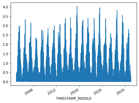
xlabel = f"{var} ({units})"
xlim = [series.min(), series.max()]

Stats

Overall mean

_yearly_avg = series.resample('YE').mean()
_overall_mean = _yearly_avg.mean()
_overall_sd = _yearly_avg.std()
print(f"Overall mean: {_overall_mean} +/- {_overall_sd}")

Overall mean: 0.3552420731579419 +/- 0.04715788745007997

Yearly means

ym = series.resample('YE').mean()
ym

TIMESTAMP_MIDDLE
2005-12-31    0.346331
2006-12-31    0.359115
2007-12-31    0.335538
2008-12-31    0.306914
2009-12-31    0.334010
2010-12-31    0.302139
2011-12-31    0.381283
2012-12-31    0.322967
2013-12-31    0.311386
2014-12-31    0.323487
2015-12-31    0.415564
2016-12-31    0.340576
2017-12-31    0.378826
2018-12-31    0.424159
2019-12-31    0.409711
2020-12-31    0.404670
2021-12-31    0.290171
2022-12-31    0.438485
2023-12-31    0.391231
2024-12-31    0.288277
Freq: YE-DEC, Name: VPD_T1_47_1, dtype: float64

ym.sort_values(ascending=False)

TIMESTAMP_MIDDLE
2022-12-31    0.438485
2018-12-31    0.424159
2015-12-31    0.415564
2019-12-31    0.409711
2020-12-31    0.404670
2023-12-31    0.391231
2011-12-31    0.381283
2017-12-31    0.378826
2006-12-31    0.359115
2005-12-31    0.346331
2016-12-31    0.340576
2007-12-31    0.335538
2009-12-31    0.334010
2014-12-31    0.323487
2012-12-31    0.322967
2013-12-31    0.311386
2008-12-31    0.306914
2010-12-31    0.302139
2021-12-31    0.290171
2024-12-31    0.288277
Name: VPD_T1_47_1, dtype: float64

Monthly averages

seriesdf = pd.DataFrame(series)
seriesdf['MONTH'] = seriesdf.index.month
seriesdf['YEAR'] = seriesdf.index.year
monthly_avg = seriesdf.groupby(['YEAR', 'MONTH'])[varname].mean().unstack()
monthly_avg

MONTH	1	2	3	4	5	6	7	8	9	10	11	12
YEAR
2005	0.098728	0.071203	0.255526	0.368644	0.566865	0.826770	0.667390	0.451273	0.419682	0.241639	0.130418	0.038538
2006	0.065026	0.077202	0.125051	0.296425	0.418049	0.762348	1.136930	0.319461	0.448141	0.285055	0.238983	0.119354
2007	0.097568	0.151464	0.228125	0.798676	0.527100	0.484729	0.570716	0.469590	0.342726	0.202463	0.094519	0.053188
2008	0.156523	0.209550	0.180537	0.242362	0.625697	0.534153	0.644119	0.493965	0.257575	0.174711	0.103464	0.050405
2009	0.055331	0.095297	0.154754	0.515293	0.578902	0.487260	0.604620	0.783934	0.410350	0.234502	0.146221	0.067759
2010	0.031270	0.115490	0.262697	0.478771	0.275770	0.596658	0.734554	0.434073	0.368292	0.210315	0.104567	0.051532
2011	0.074444	0.160941	0.304421	0.665664	0.720928	0.539708	0.542076	0.721999	0.456061	0.173393	0.143382	0.060903
2012	0.047402	0.096555	0.436990	0.345349	0.541762	0.526567	0.529450	0.644753	0.338462	0.188343	0.112636	0.060602
2013	0.044530	0.040868	0.151234	0.300698	0.236430	0.563825	0.927837	0.680899	0.355528	0.195319	0.076643	0.150297
2014	0.089826	0.133849	0.381018	0.414037	0.427751	0.841078	0.476376	0.396185	0.335520	0.206614	0.106579	0.067637
2015	0.080089	0.086698	0.288041	0.517502	0.444502	0.654488	1.181111	0.875660	0.382253	0.147485	0.176234	0.124083
2016	0.163168	0.073469	0.194694	0.271803	0.471009	0.361981	0.714703	0.749679	0.579225	0.145200	0.120538	0.104775
2017	0.027242	0.131541	0.346825	0.418633	0.621429	0.818097	0.717419	0.727567	0.305520	0.304060	0.092604	0.014897
2018	0.048989	0.033899	0.134523	0.690992	0.466109	0.575210	1.045025	0.955584	0.618676	0.370566	0.094623	0.027068
2019	0.035984	0.260537	0.324951	0.416678	0.317199	0.903075	1.006291	0.675062	0.442672	0.177969	0.083475	0.098477
2020	0.093285	0.197273	0.266215	0.770265	0.566880	0.471992	0.916620	0.799875	0.474777	0.145026	0.108674	0.038461
2021	0.034762	0.217407	0.314375	0.445382	0.327642	0.648965	0.400432	0.399979	0.438516	0.208789	0.037754	0.014229
2022	0.075574	0.150512	0.514989	0.368359	0.598409	0.775528	1.144731	0.910807	0.308749	0.252991	0.084683	0.041637
2023	0.056557	0.152780	0.241544	0.200306	0.383447	1.009227	0.773765	0.756753	0.634094	0.384954	0.038167	0.053353
2024	0.059489	0.127057	0.251946	0.449865	0.342013	0.398504	0.634605	0.760310	0.267576	0.072583	0.053014	0.041320

Number of days below …

# plotdf = df[[varname]].copy()
# plotdf = plotdf.resample('D').min()
# belowzero = plotdf.loc[plotdf[varname] < 0].copy()
# belowzero = belowzero.groupby(belowzero.index.year).count()
# belowzero["YEAR"] = belowzero.index
# belowzero
# belowzero.plot.bar(x="YEAR", y=varname, title=f"Number of days with {varname} < 0°");
# display(belowzero)
# print(f"Average per year: {belowzero[varname].mean()} +/- {belowzero[varname].std():.2f} SD")

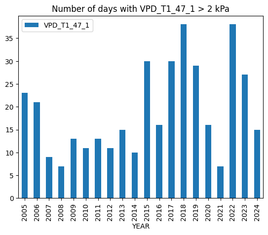
Number of days above …

plotdf = df[[varname]].copy()
plotdf = plotdf.resample('D').max()
above = plotdf.loc[plotdf[varname] > 2].copy()
above = above.groupby(above.index.year).count()
above["YEAR"] = above.index
above.plot.bar(x="YEAR", y=varname, title=f"Number of days with {varname} > 2 {units}");
display(above)
print(f"Average per year: {above[varname].mean()} +/- {above[varname].std():.2f} SD")

	VPD_T1_47_1	YEAR
TIMESTAMP_MIDDLE
2005	23	2005
2006	21	2006
2007	9	2007
2008	7	2008
2009	13	2009
2010	11	2010
2011	13	2011
2012	11	2012
2013	15	2013
2014	10	2014
2015	30	2015
2016	16	2016
2017	30	2017
2018	38	2018
2019	29	2019
2020	16	2020
2021	7	2021
2022	38	2022
2023	27	2023
2024	15	2024

Average per year: 18.95 +/- 9.91 SD

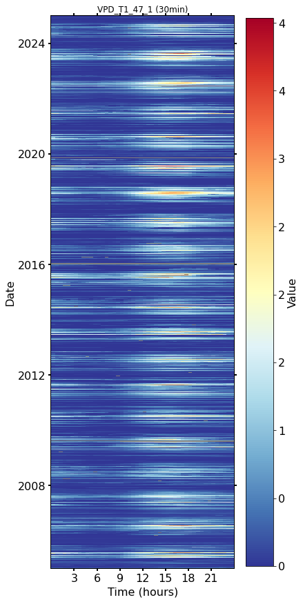
Heatmap plots

Half-hourly

fig, axs = plt.subplots(ncols=1, figsize=(6, 12), dpi=72, layout="constrained")
dv.heatmapdatetime(series=series, ax=axs, cb_digits_after_comma=0).plot()

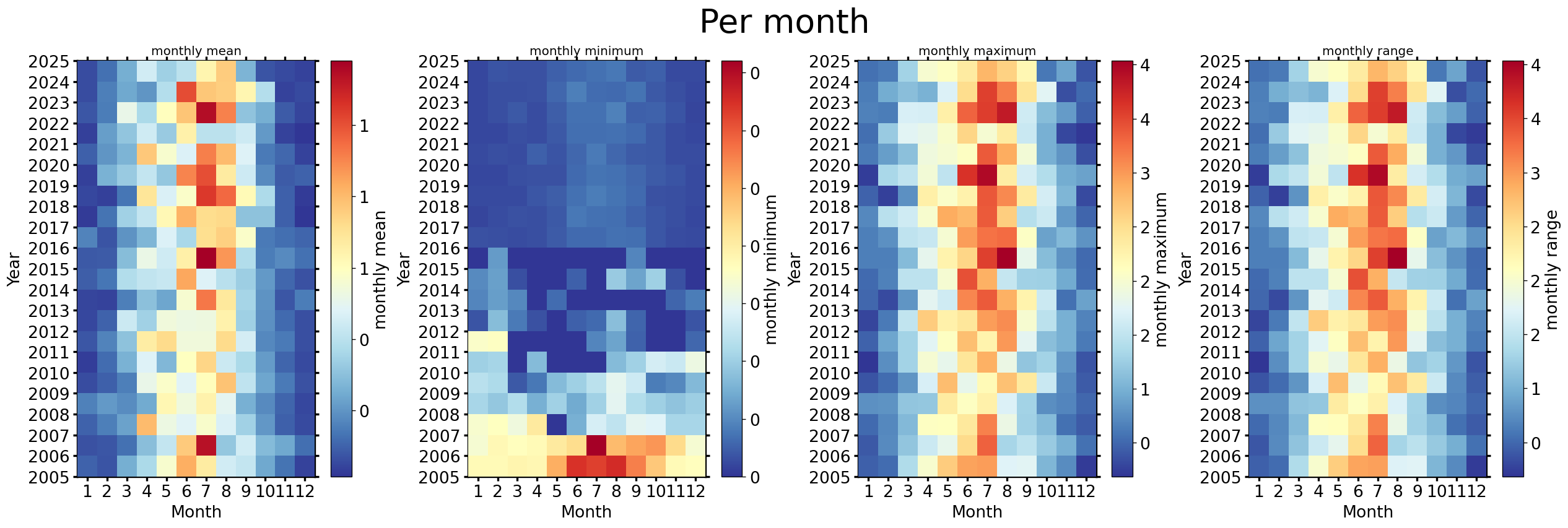
Monthly

fig, axs = plt.subplots(ncols=4, figsize=(21, 7), dpi=120, layout="constrained")
fig.suptitle(f'Per month', fontsize=32)
dv.heatmapyearmonth(series_monthly=series.resample('M').mean(), title="monthly mean", ax=axs[0], cb_digits_after_comma=0, zlabel="monthly mean").plot()
dv.heatmapyearmonth(series_monthly=series.resample('M').min(), title="monthly minimum", ax=axs[1], cb_digits_after_comma=0, zlabel="monthly minimum").plot()
dv.heatmapyearmonth(series_monthly=series.resample('M').max(), title="monthly maximum", ax=axs[2], cb_digits_after_comma=0, zlabel="monthly maximum").plot()
_range = series.resample('M').max().sub(series.resample('M').min())
dv.heatmapyearmonth(series_monthly=_range, title="monthly range", ax=axs[3], cb_digits_after_comma=0, zlabel="monthly range").plot()

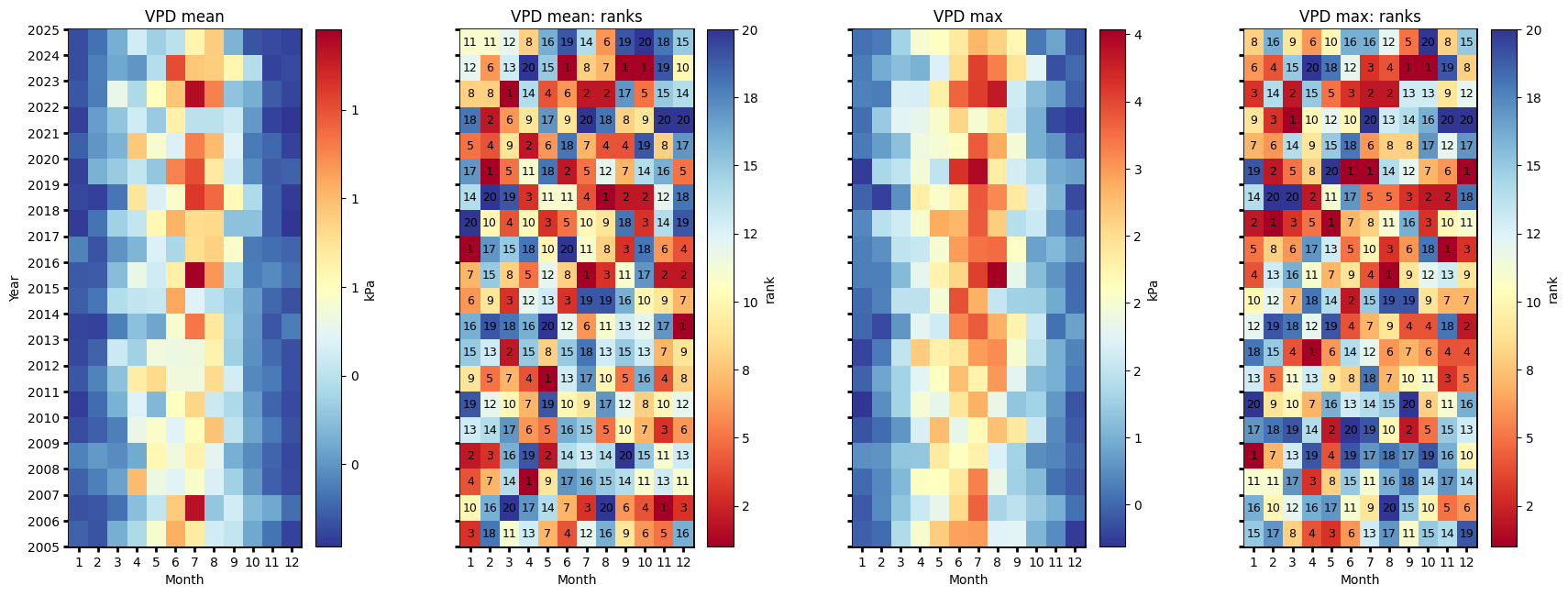
Monthly ranks

# Figure
fig = plt.figure(facecolor='white', figsize=(17, 6))

# Gridspec for layout
gs = gridspec.GridSpec(1, 4)  # rows, cols
gs.update(wspace=0.35, hspace=0.3, left=0.03, right=0.97, top=0.97, bottom=0.03)
ax_mean = fig.add_subplot(gs[0, 0])
ax_mean_ranks = fig.add_subplot(gs[0, 1])
ax_max = fig.add_subplot(gs[0, 2])
ax_max_ranks = fig.add_subplot(gs[0, 3])
params = {'axlabels_fontsize': 10, 'ticks_labelsize': 10, 'cb_labelsize': 10}
dv.heatmapyearmonth_ranks(ax=ax_mean, series=series, agg='mean', ranks=False, zlabel=units, cmap="RdYlBu_r", show_values=False, **params).plot()

hm_mean_ranks = dv.heatmapyearmonth_ranks(ax=ax_mean_ranks, series=series, agg='mean', show_values=True, **params)
hm_mean_ranks.plot()

dv.heatmapyearmonth_ranks(ax=ax_max, series=series, agg='max', ranks=False, zlabel=units, cmap="RdYlBu_r", show_values=False, **params).plot()
dv.heatmapyearmonth_ranks(ax=ax_max_ranks, series=series, agg='max', show_values=True, **params).plot()

ax_mean.set_title(f"{var} mean", color='black')
ax_mean_ranks.set_title(f"{var} mean: ranks", color='black')
ax_max.set_title(f"{var} max", color='black')
ax_max_ranks.set_title(f"{var} max: ranks", color='black')

ax_mean.tick_params(left=True, right=False, top=False, bottom=True,
                    labelleft=True, labelright=False, labeltop=False, labelbottom=True)
ax_mean_ranks.tick_params(left=True, right=False, top=False, bottom=True,
                   labelleft=False, labelright=False, labeltop=False, labelbottom=True)
ax_max.tick_params(left=True, right=False, top=False, bottom=True,
                     labelleft=False, labelright=False, labeltop=False, labelbottom=True)
ax_max_ranks.tick_params(left=True, right=False, top=False, bottom=True,
                     labelleft=False, labelright=False, labeltop=False, labelbottom=True)

ax_mean_ranks.set_ylabel("")
ax_max.set_ylabel("")
ax_max_ranks.set_ylabel("")

fig.show()

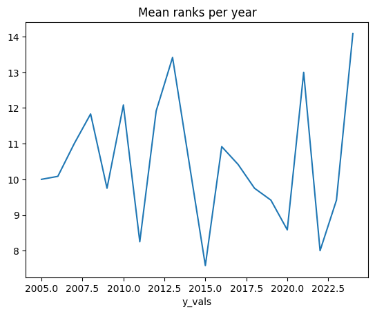
Mean ranks per year

hm_mean_ranks.hm.get_plot_data().mean(axis=1).plot(title="Mean ranks per year");

Ridgeline plots

Yearly

# rp = dv.ridgeline(series=series)
# rp.plot(
#     how='yearly',
#     kd_kwargs=None,  # params from scikit KernelDensity as dict
#     xlim=xlim,  # min/max as list
#     ylim=[0, 0.50],  # min/max as list
#     hspace=-0.8,  # overlap between months
#     xlabel=f"{var} ({units})",
#     fig_width=5,
#     fig_height=9,
#     shade_percentile=0.5,
#     show_mean_line=False,
#     fig_title=f"{var} per year (2005-2024)",
#     fig_dpi=72,
#     showplot=True,
#     ascending=False
# )

Monthly

# rp.plot(
#     how='monthly',
#     kd_kwargs=None,  # params from scikit KernelDensity as dict
#     xlim=xlim,  # min/max as list
#     ylim=[0, 0.14],  # min/max as list
#     hspace=-0.6,  # overlap between months
#     xlabel=f"{var} ({units})",
#     fig_width=4.5,
#     fig_height=8,
#     shade_percentile=0.5,
#     show_mean_line=False,
#     fig_title=f"{var} per month (2005-2024)",
#     fig_dpi=72,
#     showplot=True,
#     ascending=False
# )

Weekly

# rp.plot(
#     how='weekly',
#     kd_kwargs=None,  # params from scikit KernelDensity as dict
#     xlim=xlim,  # min/max as list
#     ylim=[0, 0.15],  # min/max as list
#     hspace=-0.6,  # overlap
#     xlabel=f"{var} ({units})",
#     fig_width=6,
#     fig_height=16,
#     shade_percentile=0.5,
#     show_mean_line=False,
#     fig_title=f"{var} per week (2005-2024)",
#     fig_dpi=72,
#     showplot=True,
#     ascending=False
# )

Single years per month

# uniq_years = series.index.year.unique()
# for uy in uniq_years:
#     series_yr = series.loc[series.index.year == uy].copy()
#     rp = dv.ridgeline(series=series_yr)
#     rp.plot(
#         how='monthly',
#         kd_kwargs=None,  # params from scikit KernelDensity as dict
#         xlim=xlim,  # min/max as list
#         ylim=[0, 0.18],  # min/max as list
#         hspace=-0.6,  # overlap
#         xlabel=f"{var} ({units})",
#         fig_width=6,
#         fig_height=7,
#         shade_percentile=0.5,
#         show_mean_line=False,
#         fig_title=f"{var} per month ({uy})",
#         fig_dpi=72,
#         showplot=True,
#         ascending=False
#     )

Single years per week

# uniq_years = series.index.year.unique()
# for uy in uniq_years:
#     series_yr = series.loc[series.index.year == uy].copy()
#     rp = dv.ridgeline(series=series_yr)
#     rp.plot(
#         how='weekly',
#         kd_kwargs=None,  # params from scikit KernelDensity as dict
#         xlim=xlim,  # min/max as list
#         ylim=[0, 0.3],  # min/max as list
#         hspace=-0.8,  # overlap
#         xlabel=f"{var} ({units})",
#         fig_width=9,
#         fig_height=18,
#         shade_percentile=0.5,
#         show_mean_line=False,
#         fig_title=f"{var} per week ({uy})",
#         fig_dpi=72,
#         showplot=True,
#         ascending=False
#     )

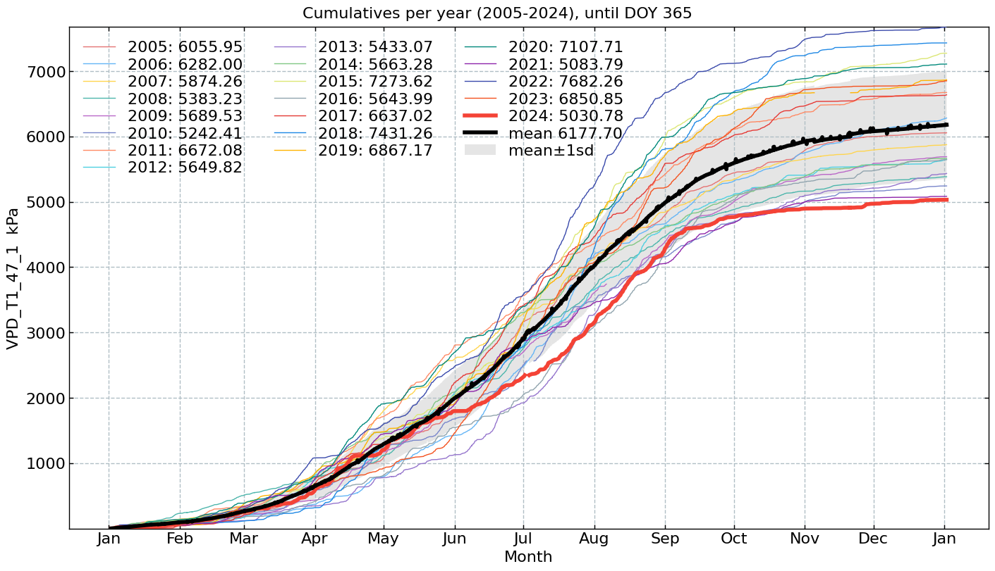
Cumulative plot

CumulativeYear(
    series=series,
    series_units=units,
    start_year=2005,
    end_year=2024,
    show_reference=True,
    excl_years_from_reference=None,
    highlight_year=2024,
    highlight_year_color='#F44336').plot();

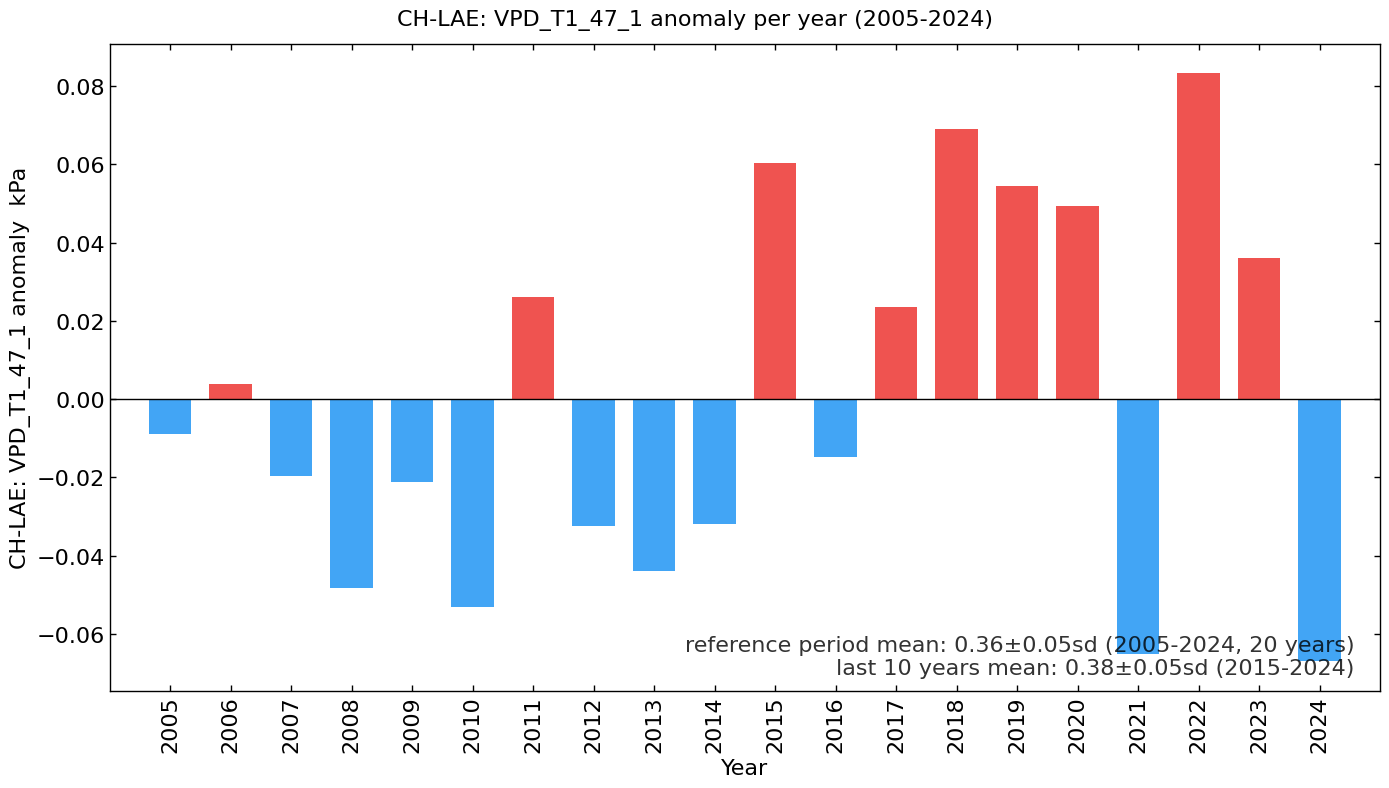
Long-term anomalies

series_yearly_mean = series.resample('YE').mean()
series_yearly_mean.index = series_yearly_mean.index.year
series_label = f"CH-LAE: {varname}"
LongtermAnomaliesYear(series=series_yearly_mean,
                      series_label=series_label,
                      series_units=units,
                      reference_start_year=2005,
                      reference_end_year=2024).plot()

End of notebook

dt_string = datetime.now().strftime("%Y-%m-%d %H:%M:%S")
print(f"Finished. {dt_string}")

Finished. 2025-06-12 00:54:40