Level-0: Preliminary flux calculations#
Info
Results from preliminary flux calculations with relaxed processing settings assist in finding the most appropriate settings for final flux calculations (Level-1).
Level-0 flux results help to find the best settings for the final flux calculations. Generally, these preliminary results are used:
to check whether the flux processing works,
to check the wind direction across years,
to determine appropriate time windows for lag search for final flux calculations.
More details can be found in the documentation of the Flux Processing Chain
OPENLAG runs to determine final lag ranges#
Notebook
The lag between turbulent departures of wind and the gas of interest was first determined in a relatively wide time window (called OPENLAG):
IRGA OPENLAG time window: between
-1sand+10s. For IRGA, the goal was to find an appropriate nominal time lag, and to determine a time window for lag search as narrow as possible.QCL OPENLAG time window: between
-1sand+10s, and a second OPENLAG run between-1sand+5s. The second OPENLAG run was done because the first run showed that the time lags accumulated in a narrower range below +5s. For QCL fluxes, constant time lags were used for the final flux calcs, so here in the OPENLAG runs it was very important to get the value for the constant lag as correct as possible. The final lag range was then set according to these narrower results.
The value
-1swas used as the starting value for the time window because EddyPro had issues with a start value of0s, in that case the lag search started e.g. at +1s for some reason (maybe bug)The results from the OPENLAG runs were used to define a time window as narrow as possible (IRGA) for the final flux calculations (Level-1)
The histograms of found OPENLAG time lags were inspected to determine whether there was a the histogram bin with peak distribution
IRGA: peak of distribution was used as nominal (default) lag, time ranges around this peak were used as time window (table)
QCL: peak of distrubution was used as constant lag for the respective time period, no time window used, all used lags were constant (table)
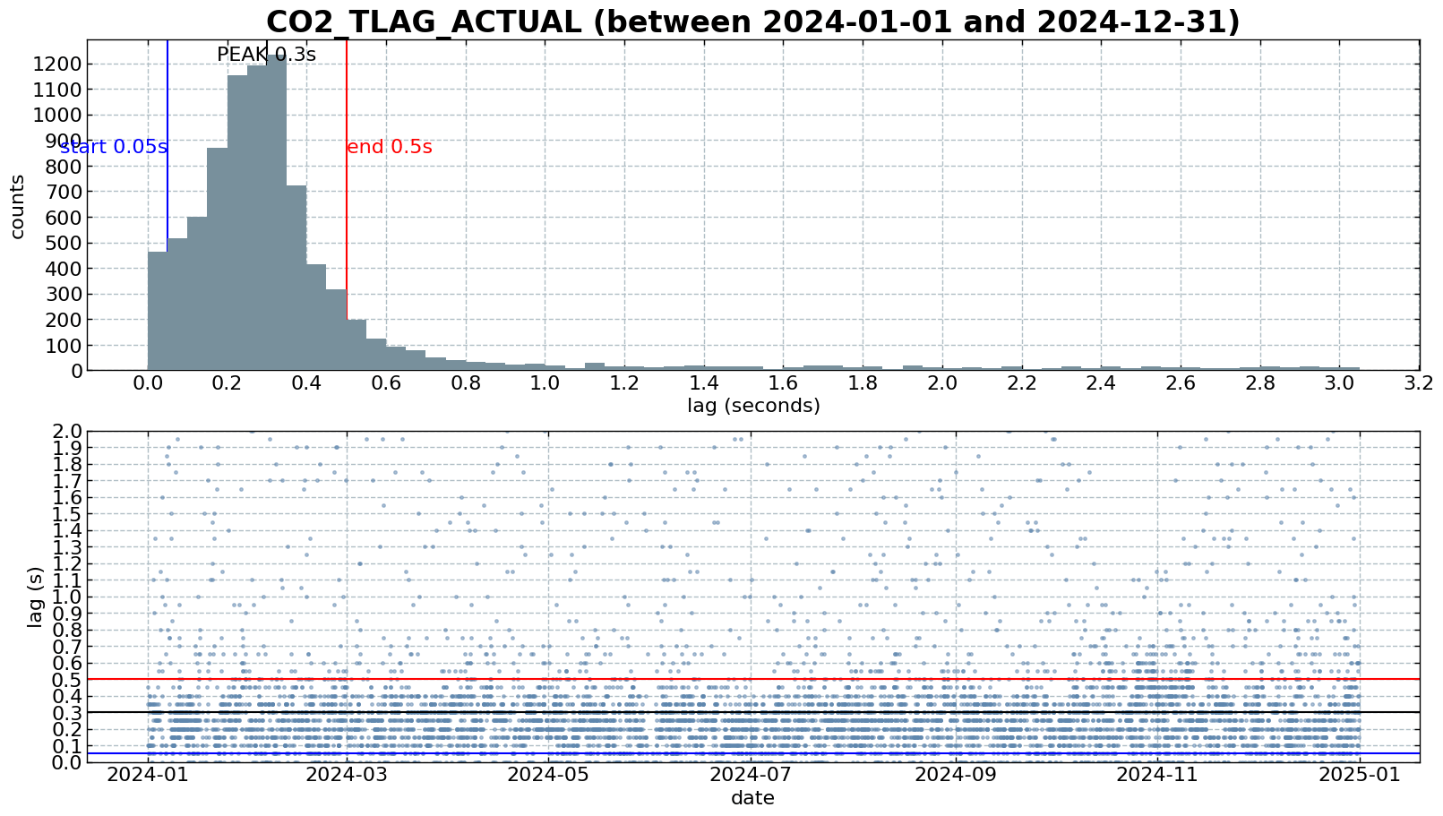
Fig. 2 Results for the OPENLAG run for CO2 (Level-0 fluxes) in 2024. The time lag between turbulent departures of vertical wind and CO2 molar densities of the open-path IRGA was first searched in a time window between -1s and 10s, then the window was narrowed down to get a clearer histogram peak for the most frequently found time lag. Level-0 flux calculations use no nominal (default) time lag, only simple covariance maximization.These results were used to define a narrow time window for final flux calculations in Level-1. In this example, for Level-1 flux calculations, the time lag with peak distribution was used as the nominal (default) time lag (0.30s), the time window for lag search was set to between +0.05s and +0.5s.#
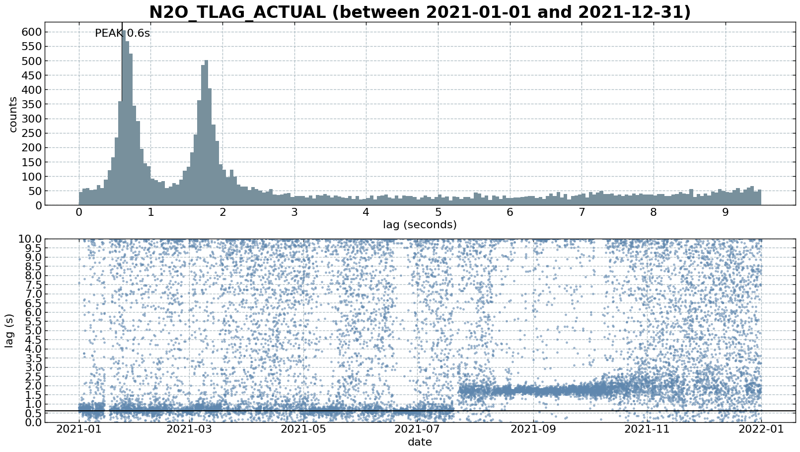
Fig. 3 Histogram and time series of found time lags between turbulent departures of vertical wind and N2O mixing ratios. Results from the OPENLAG run (Level-0 fluxes) in 2021. The histogram shows a clear bimodal distribution, which indicates that the time lag between the two scalars is not constant. In this example, there are two distinct time periods: the first time period has shorter lags and ranges from January to 22 July; the second time period has longer lags and ranges from 23 July to 31 December. In this example, the fluxes for the two time periods are calculated separately, with their own respective constant time lags. Time lags get noisier towards the end of the year due to (very) low N2O fluxes and therefore low signal-to-noise ratios. However, lags after 31 December 2021, during the following year, are still in the same range, therefore our best estimate is that the lags remain essentially the same during the noisy period.#
time period |
CO2 IRGA |
H2O IRGA |
Notes |
|---|---|---|---|
2005_X |
0.20, 0.05-0.40 |
same as CO2 |
|
2006_X |
0.25, 0.05-0.40 |
same as CO2 |
|
2007_X |
0.25, 0.05-0.40 |
same as CO2 |
|
2008_X |
0.25, 0.05-0.40 |
same as CO2 |
|
2009_X |
0.25, 0.05-0.40 |
same as CO2 |
|
2010_X |
0.30, 0.05-0.50 |
same as CO2 |
|
2011_X |
0.30, 0.05-0.55 |
same as CO2 |
|
2012_X |
0.35, 0.05-0.55 |
same as CO2 |
first time period QCL |
2013_X |
0.30, 0.05-0.55 |
same as CO2 |
|
2014_X |
0.30, 0.05-0.55 |
same as CO2 |
|
2015_X |
0.30, 0.05-0.55 |
same as CO2 |
|
2016_X |
0.35, 0.05-0.55 |
same as CO2 |
|
2017_X |
0.30, 0.05-0.55 |
same as CO2 |
|
2018_1+2+3+4 |
0.25, 0.05-0.50 |
same as CO2 |
|
2019_1+2+3+4+5 |
0.30, 0.05-0.45 |
same as CO2 |
|
2020_1+2+3+4+5 |
0.30, 0.05-0.45 |
same as CO2 |
|
2021_1+2 |
0.25, 0.05-0.45 |
same as CO2 |
|
2022_1+2+3 |
0.25, 0.05-0.45 |
same as CO2 |
|
2023_1 |
0.30, 0.05-0.50 |
same as CO2 |
|
2024_1 |
0.30, 0.05-0.50 |
same as CO2 |
time period |
N2O QCL LGR |
CH4 QCL LGR |
H2O QCL LGR |
Notes |
|---|---|---|---|---|
2012_X |
0.85, 0.70-1.50 |
0.85, 0.70-1.50 |
1.30, 1.00-3.00 |
first time period QCL |
2013_X |
1.15, 0.85-1.70 |
1.10, 0.85-1.80 |
2.10, 1.30-3.30 |
|
2014_X |
1.25, 0.95-1.60 |
1.15, 0.90-1.80 |
2.00, 1.30-3.30 |
|
2015_X |
1.35, 0.70-2.00 |
1.25, 0.70-2.00 |
1.95, 1.20-4.00 |
|
2016_2 |
0.85, 0.65-2.00 |
1.00, 0.60-2.00 |
2.45, 1.80-4.50 |
|
2016_1+3_2017_1+2 |
1.15, 0.70-1.95 |
0.95, 0.70-2.00 |
1.95, 1.50-3.30 |
2017_1+2: no H2O lag visible |
2017_3_2018_1 |
1.60, 1.20-2.35 |
1.65, 1.10-2.45 |
2.50, 1.50-4.00 |
only few data, no H2O lag visible |
2018_2 |
n.a. |
n.a. |
n.a. |
2018_2: no data for QCL |
2018_3 |
2.00, 1.25-2.55 |
2.05, 1.25-2.55 |
4.45, 4.00-6.00 |
no H2O lag visible |
2018_4_2019_1+3 |
1.45, 1.00-2.50 |
1.25, 1.00-2.50 |
n.a. |
no H2O |
2019_2 |
6.30, 4.00-10.00 |
6.80, 4.00-10.00 |
n.a. |
not clear in Mar and Apr; no H2O |
2019_4 |
1.55, 0.90-2.35 |
1.35, 0.90-2.20 |
n.a. |
no H2O |
2019_5 |
1.35, 1.00-2.50 |
1.30, 1.00-2.50 |
n.a. |
no H2O |
2020_1+2 |
1.45, 1.00-2.50 |
1.55, 1.00-2.50 |
n.a. |
no H2O |
2020_3 |
0.70, 0.40-0.90 |
0.65, 0.45-0.90 |
n.a. |
no H2O |
2020_4+5_2021_1 |
0.60, 0.40-0.90 |
0.65, 0.45-0.90 |
0.70, 0.60-2.00 |
last time period QCL, H2O available again since 2020_4 |
2021_2_2022_1 |
1.75, 1.50-3.30 |
1.75, 1.50-3.30 |
1.80, 1.65-6.00 |
LGR, lag fluctuates within these ranges |
Check wind direction across years#
Notebook
I compared histograms of wind directions between 2005 and 2024 using Level-0 fluxes and found that a sonic orientation of 7° offset to north yields very similar results across years. It is therefore possible the the sonic orientation across all years was always close to 7°.
Here are results from a comparison of annual wind direction histograms (with bin width of 1°) to a reference period (2006-2009), all wind directions were calculated with a north offset of 7°, then a histogram was calculated for each year. The OFFSET describes how many degrees have to be added (or subtracted) to the half-hourly wind direction to yield a histogram that is most similar to the reference. All OFFSETS are small, which indicates that the wind directions are in good agreement (table).
YEAR |
OFFSET (°) |
|---|---|
2005 |
1.0 |
2006 |
0.0 |
2007 |
-2.0 |
2008 |
-2.0 |
2009 |
0.0 |
2010 |
2.0 |
2011 |
6.0 |
2012 |
1.0 |
2013 |
1.0 |
2014 |
1.0 |
2015 |
1.0 |
2016 |
3.0 |
2017 |
4.0 |
2018 |
1.0 |
2019 |
-1.0 |
2020 |
-1.0 |
2021 |
-1.0 |
2022 |
1.0 |
2023 |
-2.0 |
2024 |
1.0 |