Meteo: Air temperature (TA) (2005-2024)

Author: Lukas Hörtnagl (holukas@ethz.ch)

Variable

varname = 'TA_T1_2_1'
var = "TA"  # Name shown in plots
units = "°C"

Imports

import importlib.metadata
import warnings
from datetime import datetime
from pathlib import Path
import pandas as pd
import matplotlib.pyplot as plt
import matplotlib.gridspec as gridspec

import diive as dv
from diive.core.io.files import save_parquet, load_parquet
from diive.core.plotting.cumulative import CumulativeYear
from diive.core.plotting.bar import LongtermAnomaliesYear

warnings.filterwarnings(action='ignore', category=FutureWarning)
warnings.filterwarnings(action='ignore', category=UserWarning)
version_diive = importlib.metadata.version("diive")
print(f"diive version: v{version_diive}")

diive version: v0.87.0

Load data

SOURCEDIR = r"../80_FINALIZE"
FILENAME = r"81.1_FLUXES_M15_MGMT_L4.2_NEE_GPP_RECO_LE_H_FN2O_FCH4.parquet"
FILEPATH = Path(SOURCEDIR) / FILENAME
df = load_parquet(filepath=FILEPATH)
df

Loaded .parquet file ..\80_FINALIZE\81.1_FLUXES_M15_MGMT_L4.2_NEE_GPP_RECO_LE_H_FN2O_FCH4.parquet (1.020 seconds).
    --> Detected time resolution of <30 * Minutes> / 30min 

	.PREC_RAIN_TOT_GF1_0.5_1_MEAN3H-12	.PREC_RAIN_TOT_GF1_0.5_1_MEAN3H-18	.PREC_RAIN_TOT_GF1_0.5_1_MEAN3H-24	.PREC_RAIN_TOT_GF1_0.5_1_MEAN3H-6	.SWC_GF1_0.15_1_gfXG_MEAN3H-12	.SWC_GF1_0.15_1_gfXG_MEAN3H-18	.SWC_GF1_0.15_1_gfXG_MEAN3H-24	.SWC_GF1_0.15_1_gfXG_MEAN3H-6	.TS_GF1_0.04_1_gfXG_MEAN3H-12	.TS_GF1_0.04_1_gfXG_MEAN3H-18	.TS_GF1_0.04_1_gfXG_MEAN3H-24	.TS_GF1_0.04_1_gfXG_MEAN3H-6	.TS_GF1_0.15_1_gfXG_MEAN3H-12	.TS_GF1_0.15_1_gfXG_MEAN3H-18	.TS_GF1_0.15_1_gfXG_MEAN3H-24	...	GPP_NT_CUT_50_gfRF	RECO_DT_CUT_50_gfRF	GPP_DT_CUT_50_gfRF	RECO_DT_CUT_50_gfRF_SD	GPP_DT_CUT_50_gfRF_SD	G_GF1_0.03_1	G_GF1_0.03_2	G_GF1_0.05_1	G_GF1_0.05_2	G_GF4_0.02_1	G_GF5_0.02_1	LW_OUT_T1_2_1	NETRAD_T1_2_1	PPFD_OUT_T1_2_2	SW_OUT_T1_2_1
TIMESTAMP_MIDDLE
2005-01-01 00:15:00	NaN	NaN	NaN	NaN	NaN	NaN	NaN	NaN	NaN	NaN	NaN	NaN	NaN	NaN	NaN	...	0.918553	0.093071	0.0	0.080016	0.0	NaN	NaN	NaN	NaN	NaN	NaN	NaN	NaN	NaN	NaN
2005-01-01 00:45:00	NaN	NaN	NaN	NaN	NaN	NaN	NaN	NaN	NaN	NaN	NaN	NaN	NaN	NaN	NaN	...	0.917972	0.092682	0.0	0.079688	0.0	NaN	NaN	NaN	NaN	NaN	NaN	NaN	NaN	NaN	NaN
2005-01-01 01:15:00	NaN	NaN	NaN	NaN	NaN	NaN	NaN	NaN	NaN	NaN	NaN	NaN	NaN	NaN	NaN	...	0.163001	0.093071	0.0	0.080016	0.0	NaN	NaN	NaN	NaN	NaN	NaN	NaN	NaN	NaN	NaN
2005-01-01 01:45:00	NaN	NaN	NaN	NaN	NaN	NaN	NaN	NaN	NaN	NaN	NaN	NaN	NaN	NaN	NaN	...	0.190890	0.093071	0.0	0.080016	0.0	NaN	NaN	NaN	NaN	NaN	NaN	NaN	NaN	NaN	NaN
2005-01-01 02:15:00	NaN	NaN	NaN	NaN	NaN	NaN	NaN	NaN	NaN	NaN	NaN	NaN	NaN	NaN	NaN	...	0.167042	0.092295	0.0	0.079361	0.0	NaN	NaN	NaN	NaN	NaN	NaN	NaN	NaN	NaN	NaN
...	...	...	...	...	...	...	...	...	...	...	...	...	...	...	...	...	...	...	...	...	...	...	...	...	...	...	...	...	...	...	...
2024-12-31 21:45:00	0.0	0.0	0.0	0.0	52.229004	52.226300	52.226689	52.216796	3.458828	3.150402	3.115260	3.660897	4.335667	4.347764	4.385967	...	-0.334996	1.091028	0.0	0.265808	0.0	NaN	NaN	-9.097370	-7.880106	NaN	NaN	311.167160	-5.883538	0.0	0.0
2024-12-31 22:15:00	0.0	0.0	0.0	0.0	52.227858	52.227986	52.224528	52.214211	3.522570	3.187638	3.103440	3.643396	4.338551	4.342880	4.379524	...	-0.310533	1.078751	0.0	0.264327	0.0	NaN	NaN	-9.561669	-8.172388	NaN	NaN	310.079817	-6.269816	0.0	0.0
2024-12-31 22:45:00	0.0	0.0	0.0	0.0	52.226640	52.229837	52.222456	52.209876	3.578745	3.230037	3.095339	3.624025	4.343767	4.339440	4.372636	...	-0.225651	1.079759	0.0	0.264447	0.0	NaN	NaN	-10.138718	-8.527732	NaN	NaN	309.604987	-6.934394	0.0	0.0
2024-12-31 23:15:00	0.0	0.0	0.0	0.0	52.224375	52.231151	52.221324	52.238293	3.624160	3.278488	3.093806	3.601135	4.350872	4.336333	4.366082	...	-0.558285	1.062164	0.0	0.262373	0.0	NaN	NaN	-10.649611	-8.871628	NaN	NaN	308.812117	-5.696729	0.0	0.0
2024-12-31 23:45:00	0.0	0.0	0.0	0.0	52.222007	52.230632	52.222701	52.273511	3.656167	3.331678	3.103003	3.579020	4.360311	4.334225	4.359530	...	-0.317543	1.047483	0.0	0.260688	0.0	NaN	NaN	-10.944774	-9.138224	NaN	NaN	307.372117	-8.102484	0.0	0.0

350640 rows × 812 columns

series = df[varname].copy()
series

TIMESTAMP_MIDDLE
2005-01-01 00:15:00    1.566667
2005-01-01 00:45:00    1.533333
2005-01-01 01:15:00    1.566667
2005-01-01 01:45:00    1.566667
2005-01-01 02:15:00    1.500000
                         ...   
2024-12-31 21:45:00   -1.919472
2024-12-31 22:15:00   -2.104678
2024-12-31 22:45:00   -2.089444
2024-12-31 23:15:00   -2.355761
2024-12-31 23:45:00   -2.578839
Freq: 30min, Name: TA_T1_2_1, Length: 350640, dtype: float64

xlabel = f"{var} ({units})"
xlim = [series.min(), series.max()]

Stats

Overall mean

_yearly_avg = series.resample('YE').mean()
_overall_mean = _yearly_avg.mean()
_overall_sd = _yearly_avg.std()
print(f"Overall mean: {_overall_mean} +/- {_overall_sd}")

Overall mean: 9.988191896143565 +/- 0.6491468905031849

Yearly means

ym = series.resample('YE').mean()
ym

TIMESTAMP_MIDDLE
2005-12-31     9.500346
2006-12-31     9.510808
2007-12-31    10.020665
2008-12-31     9.509768
2009-12-31     9.768376
2010-12-31     8.602752
2011-12-31     9.961233
2012-12-31     9.500586
2013-12-31     8.972617
2014-12-31    10.243456
2015-12-31    10.214341
2016-12-31     9.959387
2017-12-31    10.158153
2018-12-31    11.020365
2019-12-31    10.336325
2020-12-31    10.566112
2021-12-31     9.480925
2022-12-31    11.064683
2023-12-31    10.773193
2024-12-31    10.599748
Freq: YE-DEC, Name: TA_T1_2_1, dtype: float64

ym.sort_values(ascending=False)

TIMESTAMP_MIDDLE
2022-12-31    11.064683
2018-12-31    11.020365
2023-12-31    10.773193
2024-12-31    10.599748
2020-12-31    10.566112
2019-12-31    10.336325
2014-12-31    10.243456
2015-12-31    10.214341
2017-12-31    10.158153
2007-12-31    10.020665
2011-12-31     9.961233
2016-12-31     9.959387
2009-12-31     9.768376
2006-12-31     9.510808
2008-12-31     9.509768
2012-12-31     9.500586
2005-12-31     9.500346
2021-12-31     9.480925
2013-12-31     8.972617
2010-12-31     8.602752
Name: TA_T1_2_1, dtype: float64

Monthly averages

seriesdf = pd.DataFrame(series)
seriesdf['MONTH'] = seriesdf.index.month
seriesdf['YEAR'] = seriesdf.index.year
monthly_avg = seriesdf.groupby(['YEAR', 'MONTH'])[varname].mean().unstack()
monthly_avg

MONTH	1	2	3	4	5	6	7	8	9	10	11	12
YEAR
2005	0.210125	-0.801339	5.713844	9.710972	14.313306	18.916042	18.890143	16.856317	15.635251	10.819029	3.717182	-0.651789
2006	-2.325830	0.080485	3.055509	8.319310	13.250669	17.499912	21.749708	14.987129	16.731619	12.433040	5.730513	2.035287
2007	4.028546	3.698813	5.171103	12.285550	14.959564	17.783585	17.990020	17.422618	13.303557	9.495752	2.811688	0.882221
2008	1.432444	2.281177	4.975142	8.107183	15.310608	17.852078	18.675324	17.944528	12.829824	10.133216	3.764944	0.490034
2009	-1.625389	0.180946	4.377160	10.899647	15.477443	17.023732	18.993706	19.916496	15.428819	9.176833	6.090314	0.687469
2010	-1.816758	0.199619	4.099154	9.068338	11.873036	16.897946	19.849270	17.293014	12.834795	8.677442	5.026717	-1.278987
2011	0.892078	2.255540	5.476857	11.008608	14.657345	16.901711	16.594692	18.906124	15.817371	9.197266	4.117070	3.222475
2012	2.219987	-3.364431	6.058907	8.741281	14.288917	17.940666	18.116941	19.327690	13.941950	9.350884	5.471329	1.343973
2013	0.716500	-0.510813	2.303841	8.682419	11.226284	16.235882	20.530431	18.248934	14.630326	11.306503	4.210245	-0.573077
2014	2.091937	3.128287	5.613430	10.028926	12.870555	17.967155	17.843781	16.464852	15.091786	12.061521	6.657980	2.695666
2015	1.596828	-0.514620	5.819505	9.362186	14.146480	18.346357	21.759891	19.864031	13.115153	9.281210	6.546627	2.420249
2016	2.484183	4.107598	4.715634	8.994764	12.895846	17.391673	19.833336	18.962105	16.802195	8.680793	4.660996	-0.135555
2017	-2.624498	3.283107	7.756242	8.240388	14.695983	20.176124	19.771637	19.692754	13.370492	10.757406	4.554422	1.742608
2018	4.936138	-0.190323	3.849562	12.070434	15.426589	18.690051	20.834856	20.433843	16.170283	9.997433	5.370321	3.835440
2019	0.418184	1.984079	6.500643	8.652861	11.158806	19.701160	20.789025	18.818713	15.077914	11.575566	5.422591	3.370313
2020	1.635296	5.970656	5.577609	11.320013	13.814061	16.748215	19.583089	19.363624	15.937522	9.684012	5.287703	1.801799
2021	0.320515	2.558160	5.011026	7.622137	11.139938	18.945016	18.465003	17.840879	15.945695	8.839891	4.002620	2.687427
2022	1.159756	4.287937	5.527706	9.227786	16.238983	19.602645	20.641075	19.633025	14.191446	12.902621	6.668936	2.213690
2023	1.870183	2.294506	6.381045	8.082595	13.966407	19.479169	19.940537	19.474791	17.366343	11.646145	5.410159	2.779639
2024	1.536044	5.813781	7.137185	9.100171	13.630944	17.819154	20.193731	20.654355	14.015072	11.196474	4.607912	1.284772

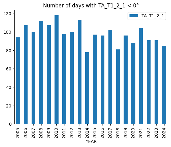
Number of days below 0°C

plotdf = df[[varname]].copy()
plotdf = plotdf.resample('D').min()
belowzero = plotdf.loc[plotdf[varname] < 0].copy()
belowzero = belowzero.groupby(belowzero.index.year).count()
belowzero["YEAR"] = belowzero.index
belowzero
belowzero.plot.bar(x="YEAR", y=varname, title=f"Number of days with {varname} < 0°");
display(belowzero)
print(f"Average per year: {belowzero[varname].mean()} +/- {belowzero[varname].std():.2f} SD")

	TA_T1_2_1	YEAR
TIMESTAMP_MIDDLE
2005	94	2005
2006	107	2006
2007	100	2007
2008	112	2008
2009	107	2009
2010	118	2010
2011	98	2011
2012	100	2012
2013	113	2013
2014	78	2014
2015	97	2015
2016	96	2016
2017	102	2017
2018	81	2018
2019	96	2019
2020	88	2020
2021	104	2021
2022	91	2022
2023	91	2023
2024	85	2024

Average per year: 97.9 +/- 10.57 SD

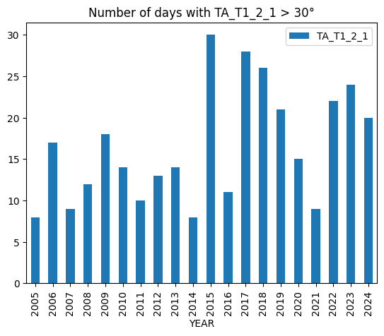
Number of days above 30°C

plotdf = df[[varname]].copy()
plotdf = plotdf.resample('D').max()
above = plotdf.loc[plotdf[varname] > 30].copy()
above = above.groupby(above.index.year).count()
above["YEAR"] = above.index
above.plot.bar(x="YEAR", y=varname, title=f"Number of days with {varname} > 30°");
display(above)
print(f"Average per year: {above[varname].mean()} +/- {above[varname].std():.2f} SD")

	TA_T1_2_1	YEAR
TIMESTAMP_MIDDLE
2005	8	2005
2006	17	2006
2007	9	2007
2008	12	2008
2009	18	2009
2010	14	2010
2011	10	2011
2012	13	2012
2013	14	2013
2014	8	2014
2015	30	2015
2016	11	2016
2017	28	2017
2018	26	2018
2019	21	2019
2020	15	2020
2021	9	2021
2022	22	2022
2023	24	2023
2024	20	2024

Average per year: 16.45 +/- 6.89 SD

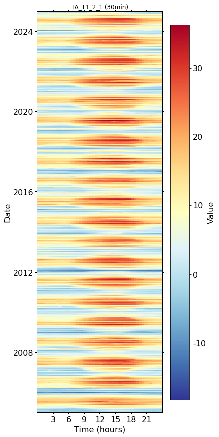
Heatmap plots

Half-hourly

fig, axs = plt.subplots(ncols=1, figsize=(6, 12), dpi=72, layout="constrained")
dv.heatmapdatetime(series=series, ax=axs, cb_digits_after_comma=0).plot()

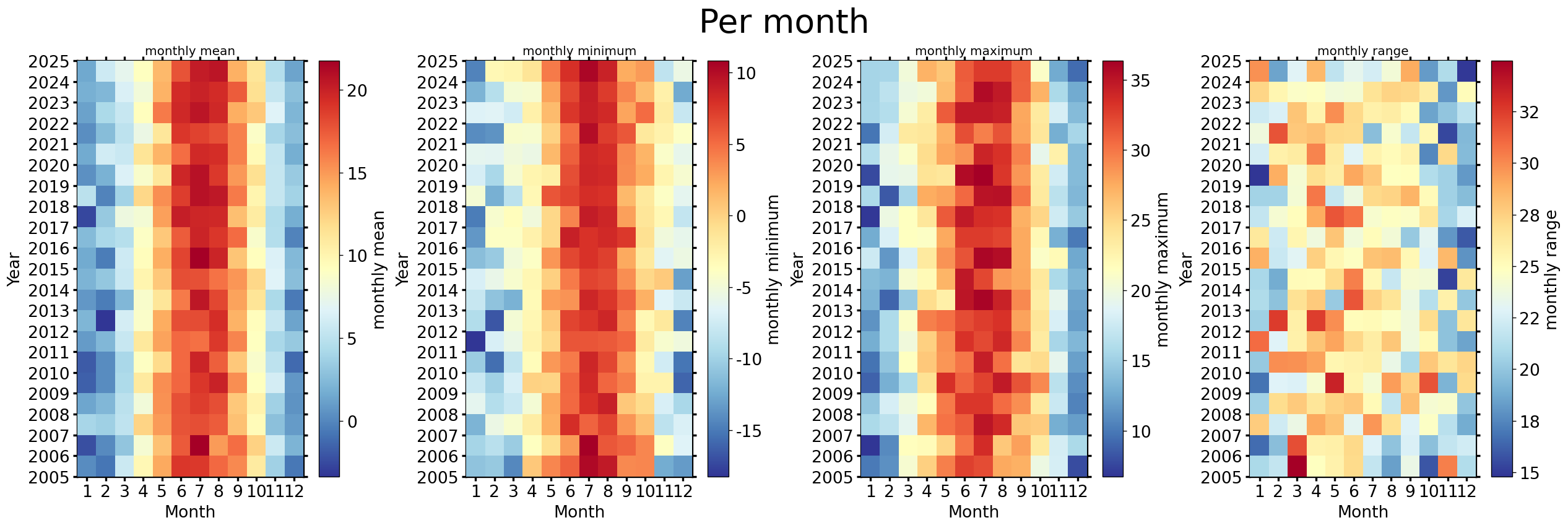
Monthly

fig, axs = plt.subplots(ncols=4, figsize=(21, 7), dpi=120, layout="constrained")
fig.suptitle(f'Per month', fontsize=32)
dv.heatmapyearmonth(series_monthly=series.resample('M').mean(), title="monthly mean", ax=axs[0], cb_digits_after_comma=0, zlabel="monthly mean").plot()
dv.heatmapyearmonth(series_monthly=series.resample('M').min(), title="monthly minimum", ax=axs[1], cb_digits_after_comma=0, zlabel="monthly minimum").plot()
dv.heatmapyearmonth(series_monthly=series.resample('M').max(), title="monthly maximum", ax=axs[2], cb_digits_after_comma=0, zlabel="monthly maximum").plot()
_range = series.resample('M').max().sub(series.resample('M').min())
dv.heatmapyearmonth(series_monthly=_range, title="monthly range", ax=axs[3], cb_digits_after_comma=0, zlabel="monthly range").plot()

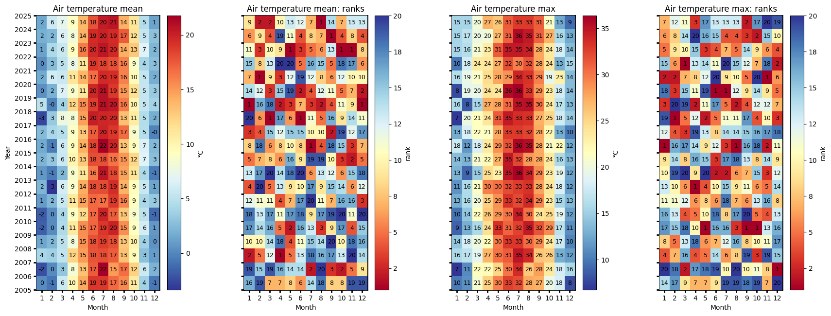
Monthly ranks

# Figure
fig = plt.figure(facecolor='white', figsize=(17, 6))

# Gridspec for layout
gs = gridspec.GridSpec(1, 4)  # rows, cols
gs.update(wspace=0.35, hspace=0.3, left=0.03, right=0.97, top=0.97, bottom=0.03)
ax_mean = fig.add_subplot(gs[0, 0])
ax_mean_ranks = fig.add_subplot(gs[0, 1])
ax_max = fig.add_subplot(gs[0, 2])
ax_max_ranks = fig.add_subplot(gs[0, 3])
params = {'axlabels_fontsize': 10, 'ticks_labelsize': 10, 'cb_labelsize': 10}
dv.heatmapyearmonth_ranks(ax=ax_mean, series=series, agg='mean', ranks=False, zlabel="°C", cmap="RdYlBu_r", show_values=True, **params).plot()

hm_mean_ranks = dv.heatmapyearmonth_ranks(ax=ax_mean_ranks, series=series, agg='mean', show_values=True, **params)
hm_mean_ranks.plot()

dv.heatmapyearmonth_ranks(ax=ax_max, series=series, agg='max', ranks=False, zlabel="°C", cmap="RdYlBu_r", show_values=True, **params).plot()
dv.heatmapyearmonth_ranks(ax=ax_max_ranks, series=series, agg='max', show_values=True, **params).plot()

ax_mean.set_title("Air temperature mean", color='black')
ax_mean_ranks.set_title("Air temperature mean: ranks", color='black')
ax_max.set_title("Air temperature max", color='black')
ax_max_ranks.set_title("Air temperature max: ranks", color='black')

ax_mean.tick_params(left=True, right=False, top=False, bottom=True,
                    labelleft=True, labelright=False, labeltop=False, labelbottom=True)
ax_mean_ranks.tick_params(left=True, right=False, top=False, bottom=True,
                   labelleft=False, labelright=False, labeltop=False, labelbottom=True)
ax_max.tick_params(left=True, right=False, top=False, bottom=True,
                     labelleft=False, labelright=False, labeltop=False, labelbottom=True)
ax_max_ranks.tick_params(left=True, right=False, top=False, bottom=True,
                     labelleft=False, labelright=False, labeltop=False, labelbottom=True)

ax_mean_ranks.set_ylabel("")
ax_max.set_ylabel("")
ax_max_ranks.set_ylabel("")

fig.show()

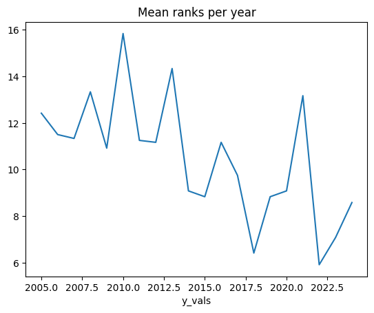
Mean ranks per year

hm_mean_ranks.hm.get_plot_data().mean(axis=1).plot(title="Mean ranks per year");

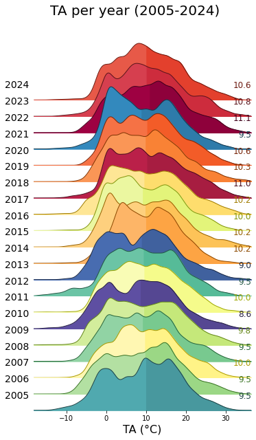
Ridgeline plots

Yearly

rp = dv.ridgeline(series=series)
rp.plot(
    how='yearly',
    kd_kwargs=None,  # params from scikit KernelDensity as dict
    xlim=xlim,  # min/max as list
    ylim=[0, 0.07],  # min/max as list
    hspace=-0.8,  # overlap between months
    xlabel=f"{var} ({units})",
    fig_width=5,
    fig_height=9,
    shade_percentile=0.5,
    show_mean_line=False,
    fig_title=f"{var} per year (2005-2024)",
    fig_dpi=72,
    showplot=True,
    ascending=False
)

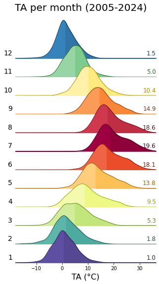
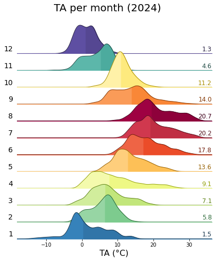
Monthly

rp.plot(
    how='monthly',
    kd_kwargs=None,  # params from scikit KernelDensity as dict
    xlim=xlim,  # min/max as list
    ylim=[0, 0.14],  # min/max as list
    hspace=-0.6,  # overlap between months
    xlabel=f"{var} ({units})",
    fig_width=4.5,
    fig_height=8,
    shade_percentile=0.5,
    show_mean_line=False,
    fig_title=f"{var} per month (2005-2024)",
    fig_dpi=72,
    showplot=True,
    ascending=False
)

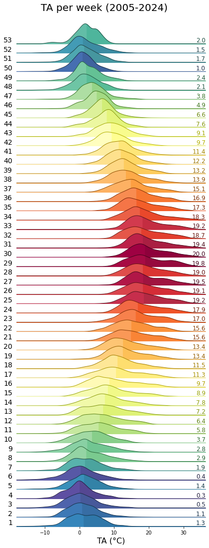
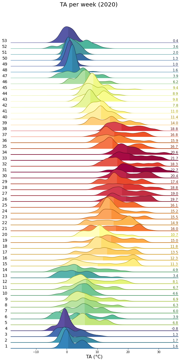
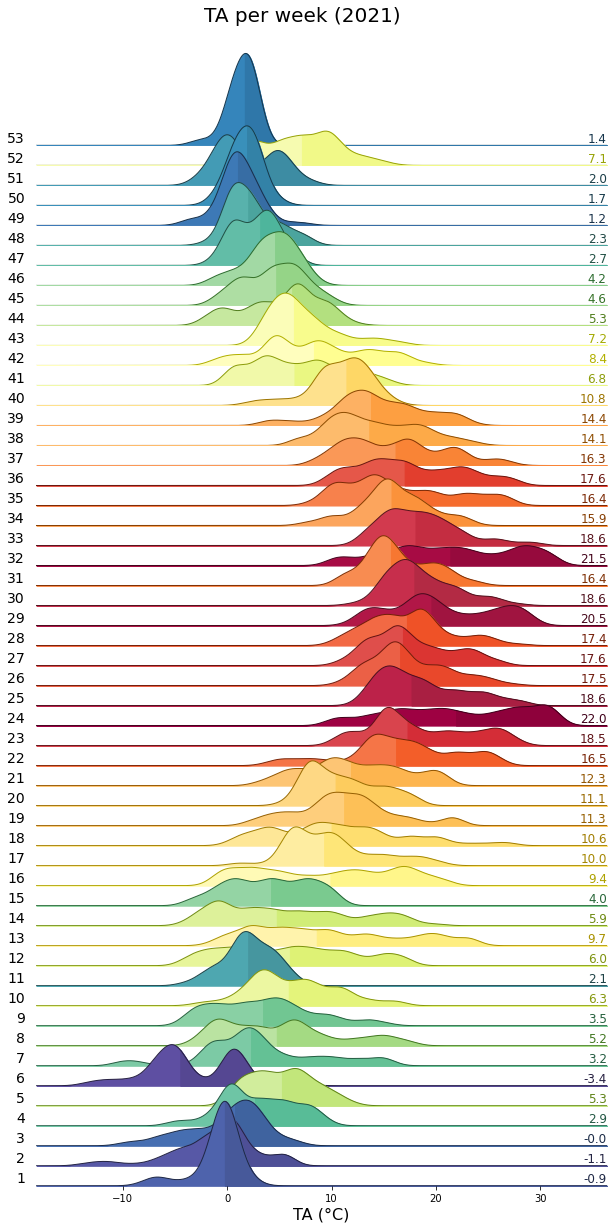
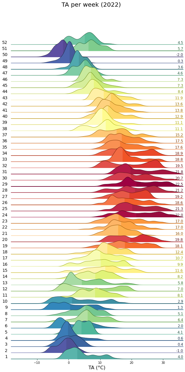
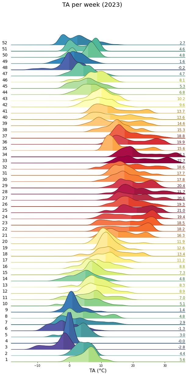
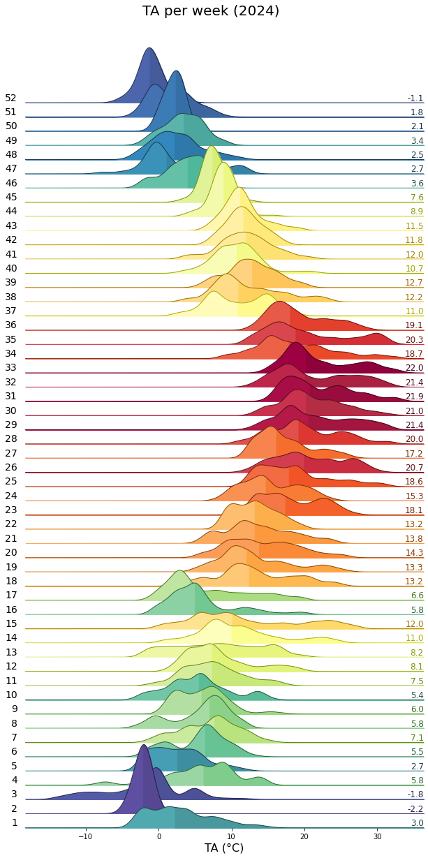
Weekly

rp.plot(
    how='weekly',
    kd_kwargs=None,  # params from scikit KernelDensity as dict
    xlim=xlim,  # min/max as list
    ylim=[0, 0.15],  # min/max as list
    hspace=-0.6,  # overlap
    xlabel=f"{var} ({units})",
    fig_width=6,
    fig_height=16,
    shade_percentile=0.5,
    show_mean_line=False,
    fig_title=f"{var} per week (2005-2024)",
    fig_dpi=72,
    showplot=True,
    ascending=False
)

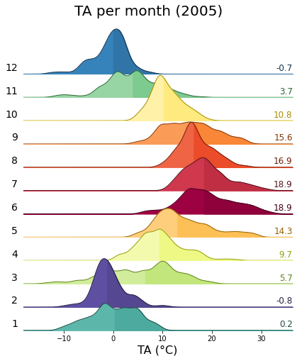
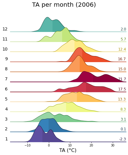
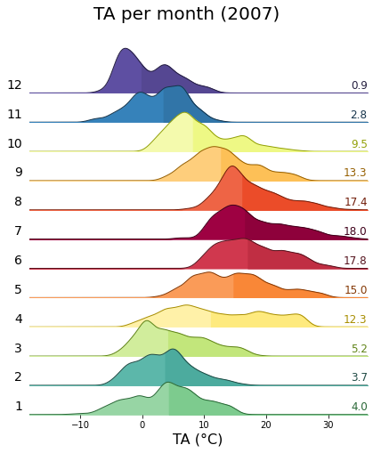
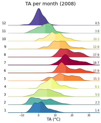
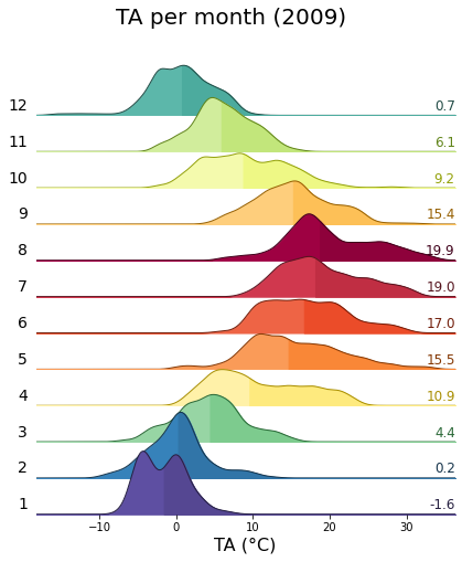
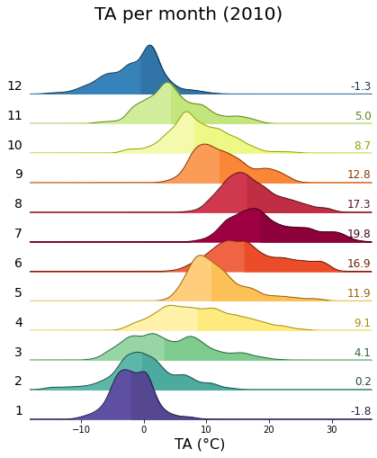
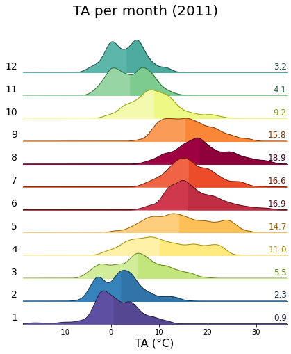
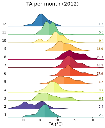
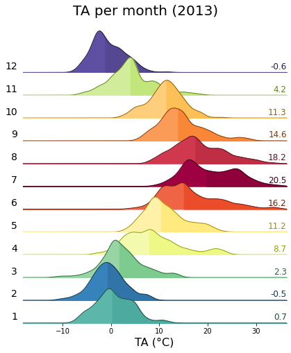
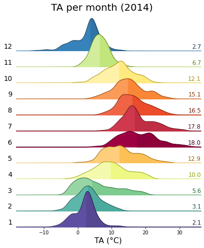
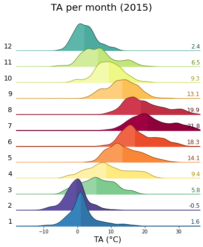
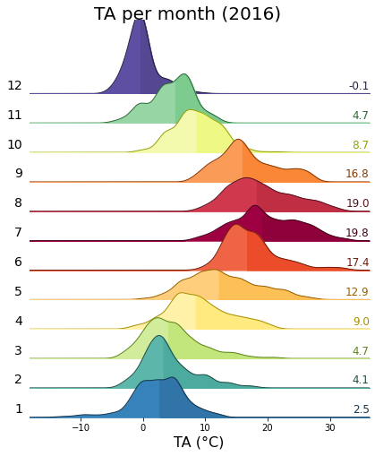
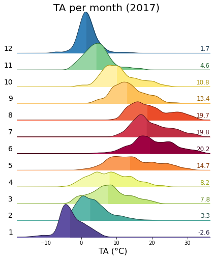
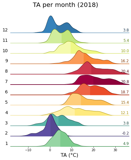
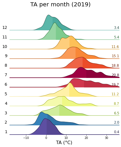
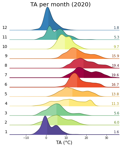
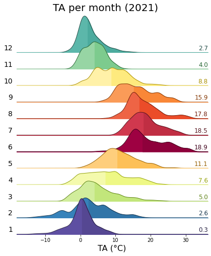
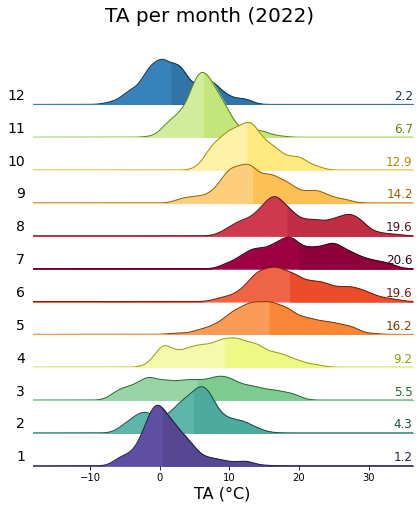
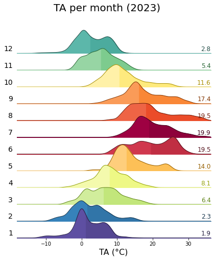
Single years per month

uniq_years = series.index.year.unique()
for uy in uniq_years:
    series_yr = series.loc[series.index.year == uy].copy()
    rp = dv.ridgeline(series=series_yr)
    rp.plot(
        how='monthly',
        kd_kwargs=None,  # params from scikit KernelDensity as dict
        xlim=xlim,  # min/max as list
        ylim=[0, 0.18],  # min/max as list
        hspace=-0.6,  # overlap
        xlabel=f"{var} ({units})",
        fig_width=6,
        fig_height=7,
        shade_percentile=0.5,
        show_mean_line=False,
        fig_title=f"{var} per month ({uy})",
        fig_dpi=72,
        showplot=True,
        ascending=False
    )

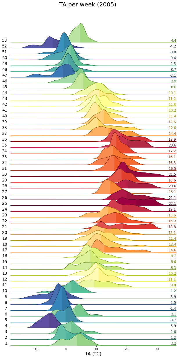
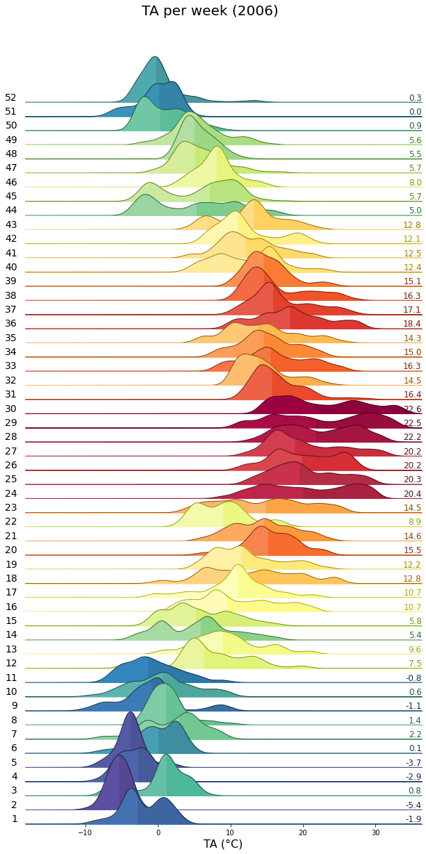
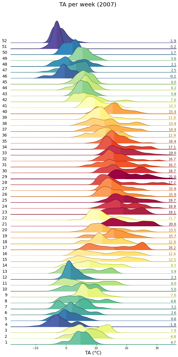
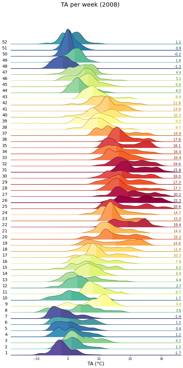
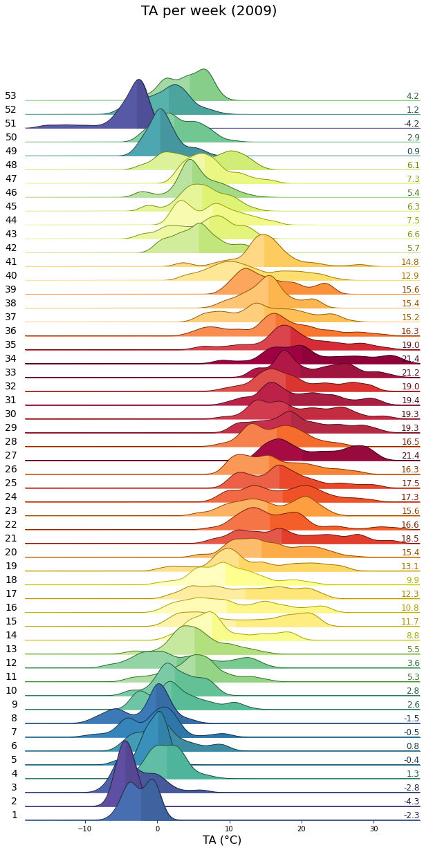
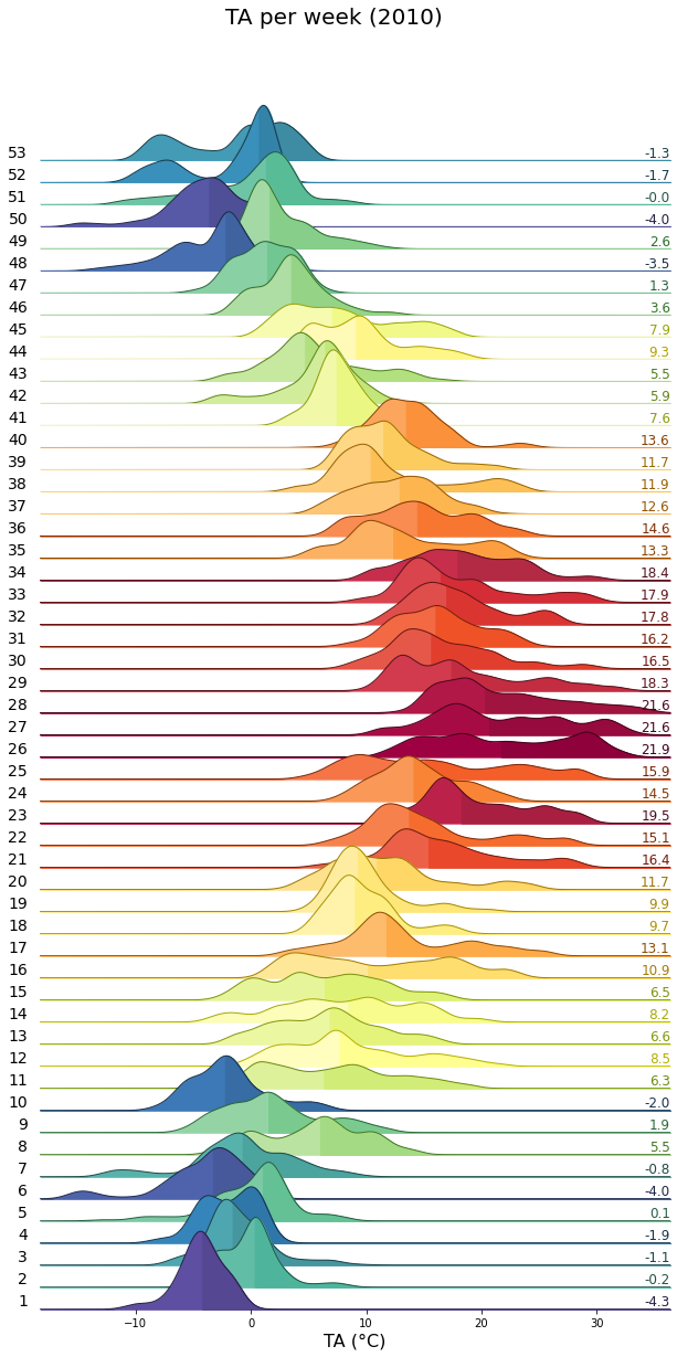
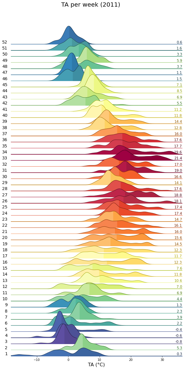
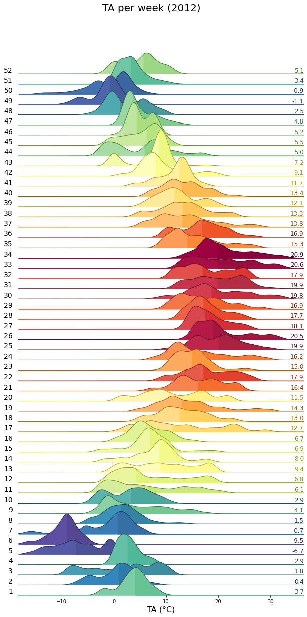
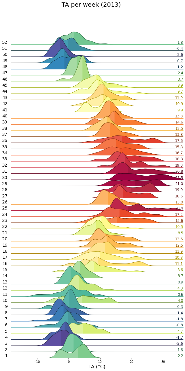
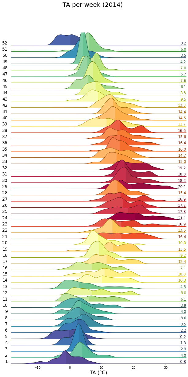
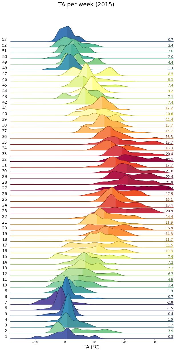
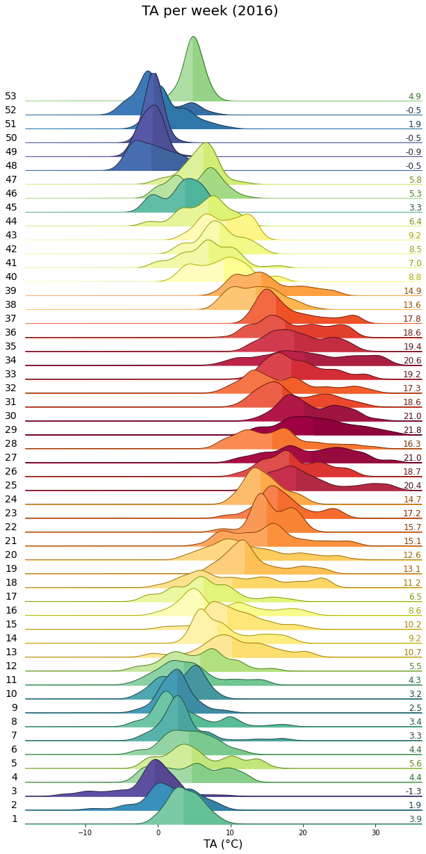
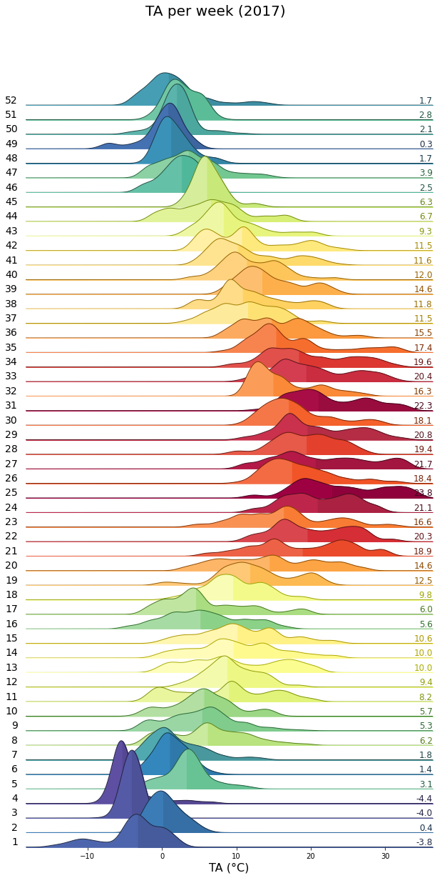
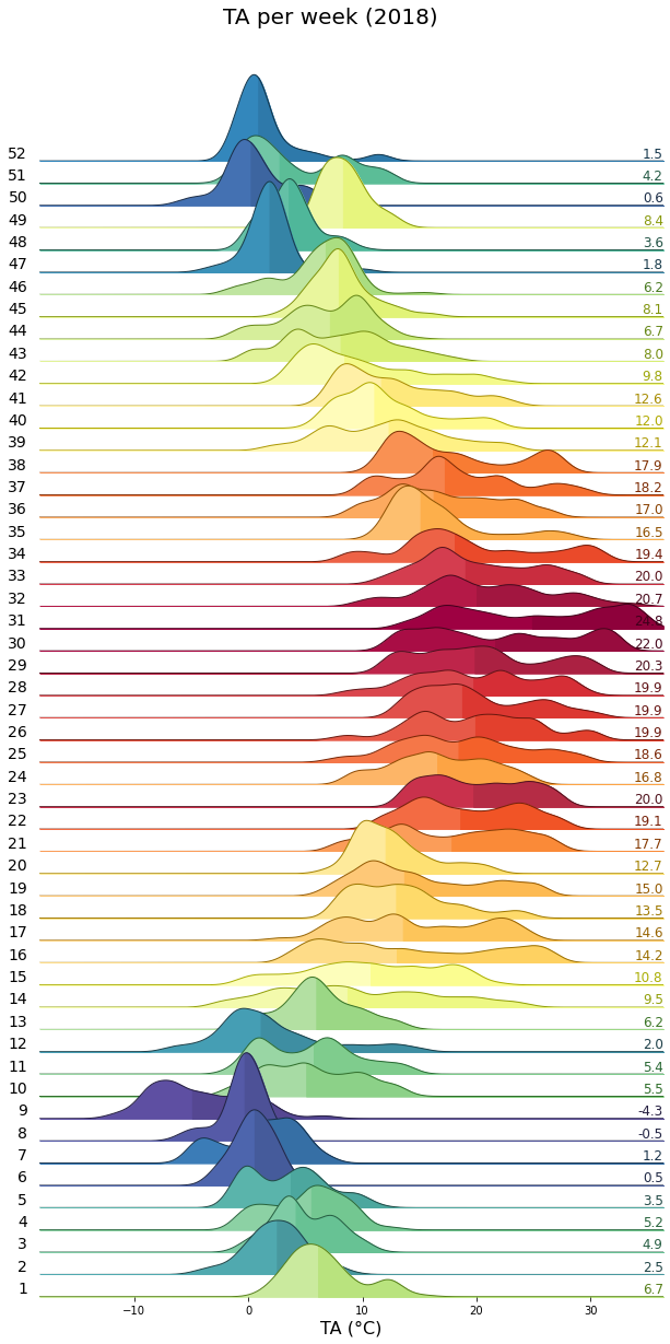
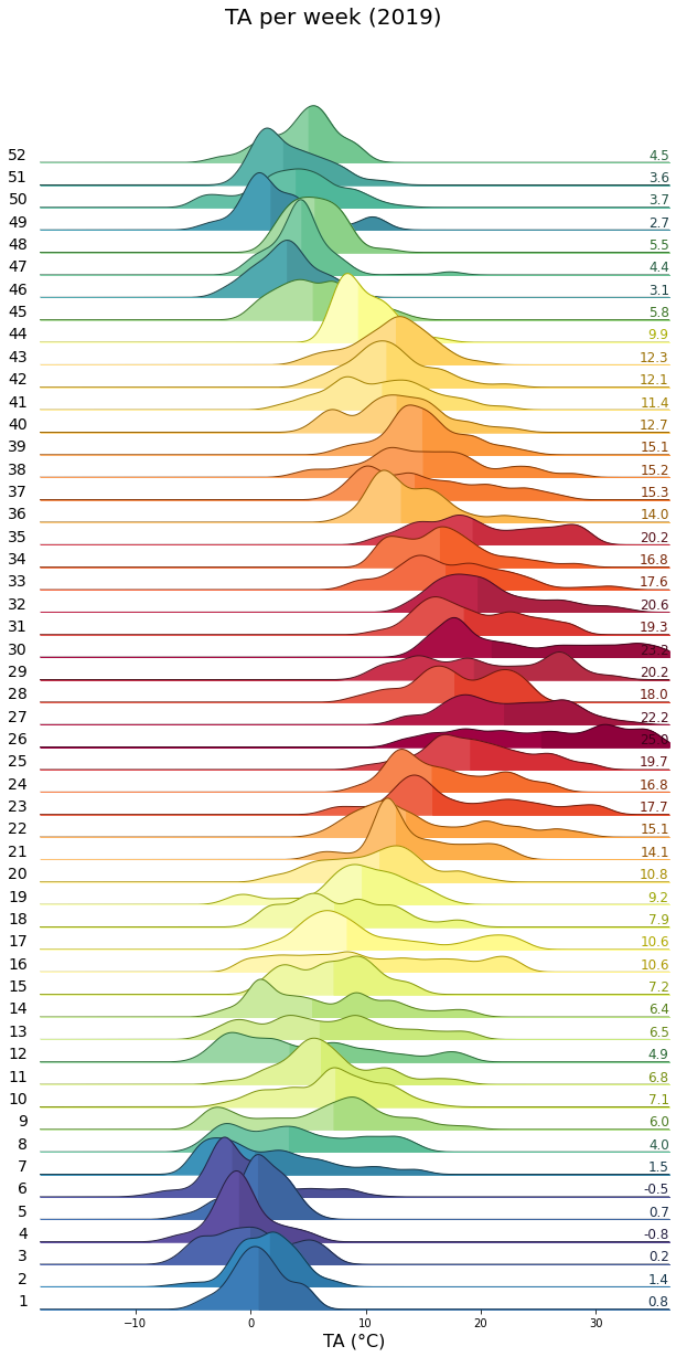
Single years per week

uniq_years = series.index.year.unique()
for uy in uniq_years:
    series_yr = series.loc[series.index.year == uy].copy()
    rp = dv.ridgeline(series=series_yr)
    rp.plot(
        how='weekly',
        kd_kwargs=None,  # params from scikit KernelDensity as dict
        xlim=xlim,  # min/max as list
        ylim=[0, 0.3],  # min/max as list
        hspace=-0.8,  # overlap
        xlabel=f"{var} ({units})",
        fig_width=9,
        fig_height=18,
        shade_percentile=0.5,
        show_mean_line=False,
        fig_title=f"{var} per week ({uy})",
        fig_dpi=72,
        showplot=True,
        ascending=False
    )

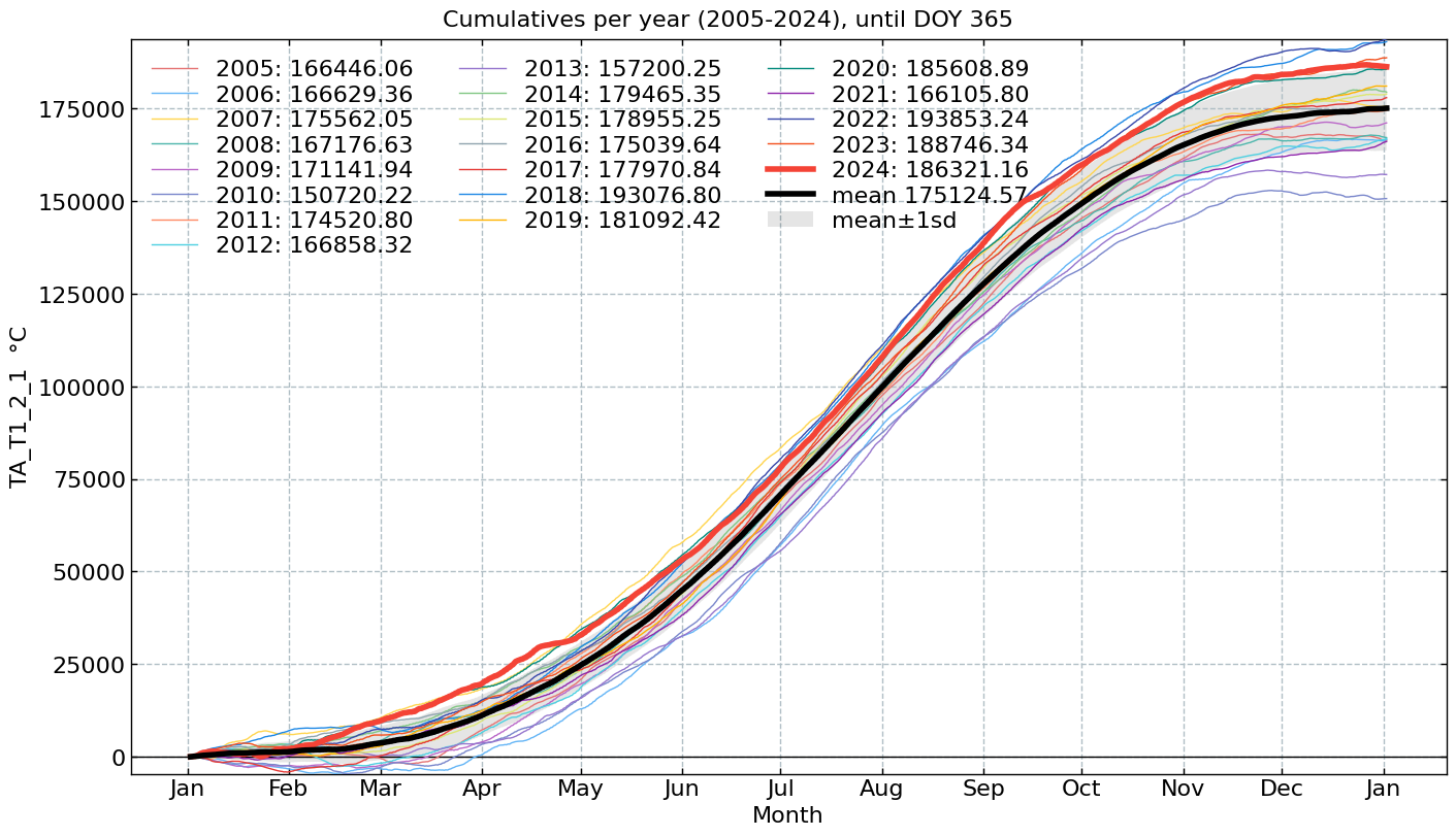
Cumulative plot

CumulativeYear(
    series=series,
    series_units=units,
    start_year=2005,
    end_year=2024,
    show_reference=True,
    excl_years_from_reference=None,
    highlight_year=2024,
    highlight_year_color='#F44336').plot();

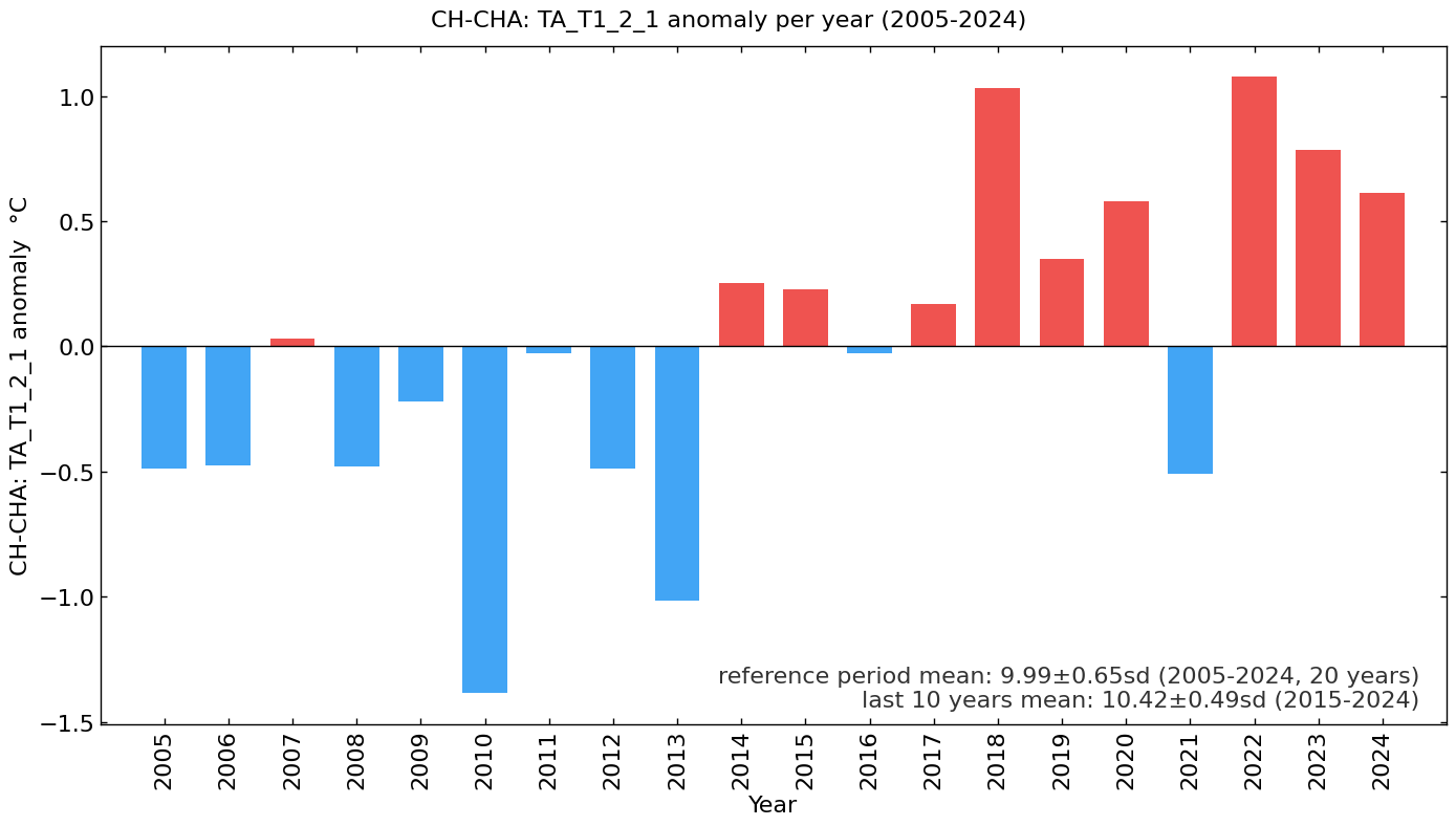
Long-term anomalies

series_yearly_mean = series.resample('YE').mean()
series_yearly_mean.index = series_yearly_mean.index.year
series_label = f"CH-CHA: {varname}"
LongtermAnomaliesYear(series=series_yearly_mean,
                      series_label=series_label,
                      series_units=units,
                      reference_start_year=2005,
                      reference_end_year=2024).plot()

End of notebook

dt_string = datetime.now().strftime("%Y-%m-%d %H:%M:%S")
print(f"Finished. {dt_string}")

Finished. 2025-05-16 12:56:46