Meteo: Air temperature (TA) (2005-2024)

Author: Lukas Hörtnagl (holukas@ethz.ch)

Variable

varname = 'VPD_T1_2_1'
var = "VPD"  # Name shown in plots
units = "kPa"

Imports

import importlib.metadata
import warnings
from datetime import datetime
from pathlib import Path
import pandas as pd
import matplotlib.pyplot as plt
import matplotlib.gridspec as gridspec

import diive as dv
from diive.core.io.files import save_parquet, load_parquet
from diive.core.plotting.cumulative import CumulativeYear
from diive.core.plotting.bar import LongtermAnomaliesYear

warnings.filterwarnings(action='ignore', category=FutureWarning)
warnings.filterwarnings(action='ignore', category=UserWarning)
version_diive = importlib.metadata.version("diive")
print(f"diive version: v{version_diive}")

diive version: v0.87.0

Load data

SOURCEDIR = r"../80_FINALIZE"
FILENAME = r"81.1_FLUXES_M15_MGMT_L4.2_NEE_GPP_RECO_LE_H_FN2O_FCH4.parquet"
FILEPATH = Path(SOURCEDIR) / FILENAME
df = load_parquet(filepath=FILEPATH)
df

Loaded .parquet file ..\80_FINALIZE\81.1_FLUXES_M15_MGMT_L4.2_NEE_GPP_RECO_LE_H_FN2O_FCH4.parquet (1.553 seconds).
    --> Detected time resolution of <30 * Minutes> / 30min 

	.PREC_RAIN_TOT_GF1_0.5_1_MEAN3H-12	.PREC_RAIN_TOT_GF1_0.5_1_MEAN3H-18	.PREC_RAIN_TOT_GF1_0.5_1_MEAN3H-24	.PREC_RAIN_TOT_GF1_0.5_1_MEAN3H-6	.SWC_GF1_0.15_1_gfXG_MEAN3H-12	.SWC_GF1_0.15_1_gfXG_MEAN3H-18	.SWC_GF1_0.15_1_gfXG_MEAN3H-24	.SWC_GF1_0.15_1_gfXG_MEAN3H-6	.TS_GF1_0.04_1_gfXG_MEAN3H-12	.TS_GF1_0.04_1_gfXG_MEAN3H-18	.TS_GF1_0.04_1_gfXG_MEAN3H-24	.TS_GF1_0.04_1_gfXG_MEAN3H-6	.TS_GF1_0.15_1_gfXG_MEAN3H-12	.TS_GF1_0.15_1_gfXG_MEAN3H-18	.TS_GF1_0.15_1_gfXG_MEAN3H-24	...	GPP_NT_CUT_50_gfRF	RECO_DT_CUT_50_gfRF	GPP_DT_CUT_50_gfRF	RECO_DT_CUT_50_gfRF_SD	GPP_DT_CUT_50_gfRF_SD	G_GF1_0.03_1	G_GF1_0.03_2	G_GF1_0.05_1	G_GF1_0.05_2	G_GF4_0.02_1	G_GF5_0.02_1	LW_OUT_T1_2_1	NETRAD_T1_2_1	PPFD_OUT_T1_2_2	SW_OUT_T1_2_1
TIMESTAMP_MIDDLE
2005-01-01 00:15:00	NaN	NaN	NaN	NaN	NaN	NaN	NaN	NaN	NaN	NaN	NaN	NaN	NaN	NaN	NaN	...	0.918553	0.093071	0.0	0.080016	0.0	NaN	NaN	NaN	NaN	NaN	NaN	NaN	NaN	NaN	NaN
2005-01-01 00:45:00	NaN	NaN	NaN	NaN	NaN	NaN	NaN	NaN	NaN	NaN	NaN	NaN	NaN	NaN	NaN	...	0.917972	0.092682	0.0	0.079688	0.0	NaN	NaN	NaN	NaN	NaN	NaN	NaN	NaN	NaN	NaN
2005-01-01 01:15:00	NaN	NaN	NaN	NaN	NaN	NaN	NaN	NaN	NaN	NaN	NaN	NaN	NaN	NaN	NaN	...	0.163001	0.093071	0.0	0.080016	0.0	NaN	NaN	NaN	NaN	NaN	NaN	NaN	NaN	NaN	NaN
2005-01-01 01:45:00	NaN	NaN	NaN	NaN	NaN	NaN	NaN	NaN	NaN	NaN	NaN	NaN	NaN	NaN	NaN	...	0.190890	0.093071	0.0	0.080016	0.0	NaN	NaN	NaN	NaN	NaN	NaN	NaN	NaN	NaN	NaN
2005-01-01 02:15:00	NaN	NaN	NaN	NaN	NaN	NaN	NaN	NaN	NaN	NaN	NaN	NaN	NaN	NaN	NaN	...	0.167042	0.092295	0.0	0.079361	0.0	NaN	NaN	NaN	NaN	NaN	NaN	NaN	NaN	NaN	NaN
...	...	...	...	...	...	...	...	...	...	...	...	...	...	...	...	...	...	...	...	...	...	...	...	...	...	...	...	...	...	...	...
2024-12-31 21:45:00	0.0	0.0	0.0	0.0	52.229004	52.226300	52.226689	52.216796	3.458828	3.150402	3.115260	3.660897	4.335667	4.347764	4.385967	...	-0.334996	1.091028	0.0	0.265808	0.0	NaN	NaN	-9.097370	-7.880106	NaN	NaN	311.167160	-5.883538	0.0	0.0
2024-12-31 22:15:00	0.0	0.0	0.0	0.0	52.227858	52.227986	52.224528	52.214211	3.522570	3.187638	3.103440	3.643396	4.338551	4.342880	4.379524	...	-0.310533	1.078751	0.0	0.264327	0.0	NaN	NaN	-9.561669	-8.172388	NaN	NaN	310.079817	-6.269816	0.0	0.0
2024-12-31 22:45:00	0.0	0.0	0.0	0.0	52.226640	52.229837	52.222456	52.209876	3.578745	3.230037	3.095339	3.624025	4.343767	4.339440	4.372636	...	-0.225651	1.079759	0.0	0.264447	0.0	NaN	NaN	-10.138718	-8.527732	NaN	NaN	309.604987	-6.934394	0.0	0.0
2024-12-31 23:15:00	0.0	0.0	0.0	0.0	52.224375	52.231151	52.221324	52.238293	3.624160	3.278488	3.093806	3.601135	4.350872	4.336333	4.366082	...	-0.558285	1.062164	0.0	0.262373	0.0	NaN	NaN	-10.649611	-8.871628	NaN	NaN	308.812117	-5.696729	0.0	0.0
2024-12-31 23:45:00	0.0	0.0	0.0	0.0	52.222007	52.230632	52.222701	52.273511	3.656167	3.331678	3.103003	3.579020	4.360311	4.334225	4.359530	...	-0.317543	1.047483	0.0	0.260688	0.0	NaN	NaN	-10.944774	-9.138224	NaN	NaN	307.372117	-8.102484	0.0	0.0

350640 rows × 812 columns

series = df[varname].copy()
series.plot(x_compat=True);
series

TIMESTAMP_MIDDLE
2005-01-01 00:15:00    0.099893
2005-01-01 00:45:00    0.097606
2005-01-01 01:15:00    0.091683
2005-01-01 01:45:00    0.071157
2005-01-01 02:15:00    0.058333
                         ...   
2024-12-31 21:45:00    0.000011
2024-12-31 22:15:00    0.000011
2024-12-31 22:45:00    0.000011
2024-12-31 23:15:00    0.000010
2024-12-31 23:45:00    0.000010
Freq: 30min, Name: VPD_T1_2_1, Length: 350640, dtype: float64

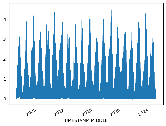
xlabel = f"{var} ({units})"
xlim = [series.min(), series.max()]

Stats

Overall mean

_yearly_avg = series.resample('YE').mean()
_overall_mean = _yearly_avg.mean()
_overall_sd = _yearly_avg.std()
print(f"Overall mean: {_overall_mean} +/- {_overall_sd}")

Overall mean: 0.31121955791661643 +/- 0.04902864837566863

Yearly means

ym = series.resample('YE').mean()
ym

TIMESTAMP_MIDDLE
2005-12-31    0.376433
2006-12-31    0.225410
2007-12-31    0.328995
2008-12-31    0.310836
2009-12-31    0.311359
2010-12-31    0.297305
2011-12-31    0.366753
2012-12-31    0.359951
2013-12-31    0.271216
2014-12-31    0.256449
2015-12-31    0.343164
2016-12-31    0.268533
2017-12-31    0.358312
2018-12-31    0.381314
2019-12-31    0.309646
2020-12-31    0.303856
2021-12-31    0.221246
2022-12-31    0.346967
2023-12-31    0.334818
2024-12-31    0.251827
Freq: YE-DEC, Name: VPD_T1_2_1, dtype: float64

ym.sort_values(ascending=False)

TIMESTAMP_MIDDLE
2018-12-31    0.381314
2005-12-31    0.376433
2011-12-31    0.366753
2012-12-31    0.359951
2017-12-31    0.358312
2022-12-31    0.346967
2015-12-31    0.343164
2023-12-31    0.334818
2007-12-31    0.328995
2009-12-31    0.311359
2008-12-31    0.310836
2019-12-31    0.309646
2020-12-31    0.303856
2010-12-31    0.297305
2013-12-31    0.271216
2016-12-31    0.268533
2014-12-31    0.256449
2024-12-31    0.251827
2006-12-31    0.225410
2021-12-31    0.221246
Name: VPD_T1_2_1, dtype: float64

Monthly averages

seriesdf = pd.DataFrame(series)
seriesdf['MONTH'] = seriesdf.index.month
seriesdf['YEAR'] = seriesdf.index.year
monthly_avg = seriesdf.groupby(['YEAR', 'MONTH'])[varname].mean().unstack()
monthly_avg

MONTH	1	2	3	4	5	6	7	8	9	10	11	12
YEAR
2005	0.133255	0.125461	0.320798	0.435624	0.631945	0.892239	0.703919	0.504649	0.379947	0.193942	0.133325	0.048627
2006	0.042295	0.079210	0.150229	0.200371	0.318859	0.548187	0.802910	0.202061	0.182587	0.095968	0.047289	0.023285
2007	0.074036	0.069035	0.159711	0.538353	0.442551	0.609129	0.679132	0.486520	0.387438	0.240121	0.143102	0.105334
2008	0.101163	0.166638	0.268867	0.270890	0.640051	0.579719	0.624814	0.467921	0.274886	0.190829	0.078831	0.054863
2009	0.054268	0.089716	0.207986	0.475443	0.553480	0.530131	0.565989	0.602001	0.351871	0.161345	0.073599	0.055018
2010	0.034755	0.114424	0.250507	0.450694	0.309132	0.641680	0.775310	0.427092	0.296411	0.141553	0.086047	0.031565
2011	0.074014	0.114899	0.251863	0.581882	0.666643	0.590370	0.568899	0.682791	0.413194	0.205884	0.090626	0.142344
2012	0.143005	0.136775	0.382794	0.406973	0.603079	0.595387	0.611613	0.677814	0.332750	0.174978	0.127317	0.113257
2013	0.094633	0.118700	0.151919	0.296454	0.270358	0.545255	0.791319	0.515140	0.281154	0.089021	0.066108	0.023130
2014	0.027523	0.072557	0.203056	0.259976	0.371139	0.634490	0.447117	0.435652	0.328777	0.173127	0.051202	0.062999
2015	0.087011	0.080146	0.237306	0.421110	0.411199	0.630129	0.951911	0.668726	0.309405	0.137561	0.119234	0.042231
2016	0.085863	0.143620	0.210320	0.261039	0.408584	0.398482	0.625289	0.506644	0.396226	0.111058	0.051096	0.017171
2017	0.063720	0.120993	0.276426	0.338306	0.588850	0.842018	0.701453	0.599454	0.311367	0.252083	0.109643	0.077889
2018	0.137392	0.107644	0.165561	0.549344	0.466748	0.671946	1.003826	0.806515	0.436501	0.138281	0.021613	0.048886
2019	0.046392	0.133999	0.290680	0.316956	0.312127	0.762132	0.866354	0.456032	0.309308	0.114732	0.041034	0.055166
2020	0.038153	0.238026	0.222998	0.550285	0.479921	0.454533	0.654878	0.533983	0.330215	0.098995	0.033549	0.011433
2021	0.026035	0.082336	0.215003	0.379660	0.336810	0.511504	0.321846	0.359091	0.292334	0.100865	0.015050	0.011092
2022	0.037497	0.151235	0.319133	0.306950	0.470408	0.627205	0.910720	0.748110	0.311619	0.149694	0.072762	0.037093
2023	0.074762	0.137025	0.220513	0.216325	0.383360	0.916441	0.648015	0.614304	0.419083	0.220624	0.100025	0.058283
2024	0.074640	0.111231	0.206013	0.344785	0.330871	0.445858	0.536684	0.562334	0.223922	0.080089	0.054793	0.043635

Number of days below …

# plotdf = df[[varname]].copy()
# plotdf = plotdf.resample('D').min()
# belowzero = plotdf.loc[plotdf[varname] < 0].copy()
# belowzero = belowzero.groupby(belowzero.index.year).count()
# belowzero["YEAR"] = belowzero.index
# belowzero
# belowzero.plot.bar(x="YEAR", y=varname, title=f"Number of days with {varname} < 0°");
# display(belowzero)
# print(f"Average per year: {belowzero[varname].mean()} +/- {belowzero[varname].std():.2f} SD")

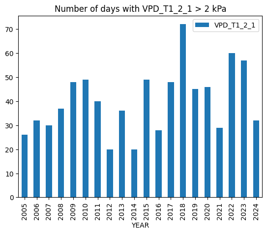
Number of days above …

plotdf = df[[varname]].copy()
plotdf = plotdf.resample('D').max()
above = plotdf.loc[plotdf[varname] > 2].copy()
above = above.groupby(above.index.year).count()
above["YEAR"] = above.index
above.plot.bar(x="YEAR", y=varname, title=f"Number of days with {varname} > 2 {units}");
display(above)
print(f"Average per year: {above[varname].mean()} +/- {above[varname].std():.2f} SD")

	VPD_T1_2_1	YEAR
TIMESTAMP_MIDDLE
2005	26	2005
2006	32	2006
2007	30	2007
2008	37	2008
2009	48	2009
2010	49	2010
2011	40	2011
2012	20	2012
2013	36	2013
2014	20	2014
2015	49	2015
2016	28	2016
2017	48	2017
2018	72	2018
2019	45	2019
2020	46	2020
2021	29	2021
2022	60	2022
2023	57	2023
2024	32	2024

Average per year: 40.2 +/- 13.72 SD

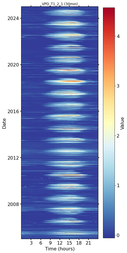
Heatmap plots

Half-hourly

fig, axs = plt.subplots(ncols=1, figsize=(6, 12), dpi=72, layout="constrained")
dv.heatmapdatetime(series=series, ax=axs, cb_digits_after_comma=0).plot()

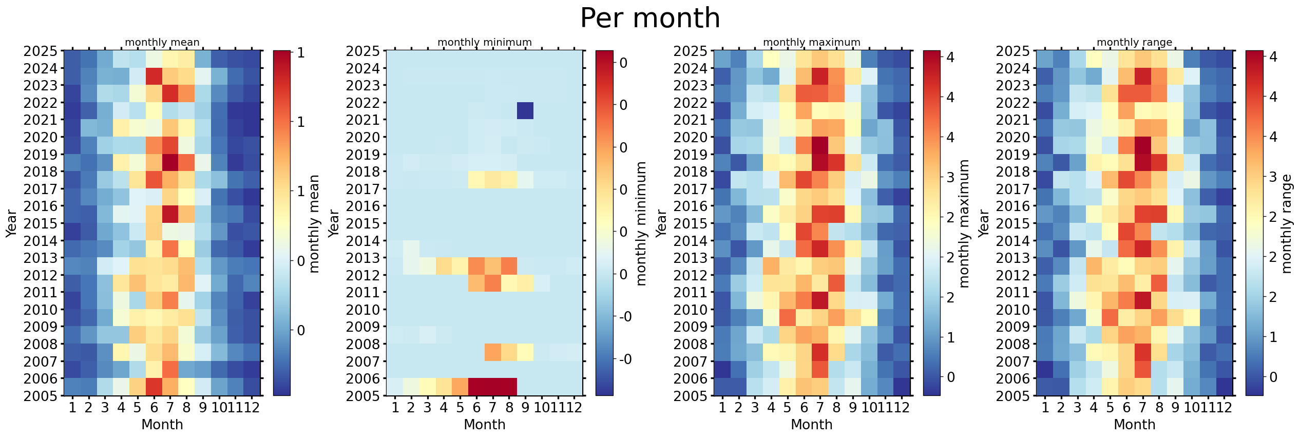
Monthly

fig, axs = plt.subplots(ncols=4, figsize=(21, 7), dpi=120, layout="constrained")
fig.suptitle(f'Per month', fontsize=32)
dv.heatmapyearmonth(series_monthly=series.resample('M').mean(), title="monthly mean", ax=axs[0], cb_digits_after_comma=0, zlabel="monthly mean").plot()
dv.heatmapyearmonth(series_monthly=series.resample('M').min(), title="monthly minimum", ax=axs[1], cb_digits_after_comma=0, zlabel="monthly minimum").plot()
dv.heatmapyearmonth(series_monthly=series.resample('M').max(), title="monthly maximum", ax=axs[2], cb_digits_after_comma=0, zlabel="monthly maximum").plot()
_range = series.resample('M').max().sub(series.resample('M').min())
dv.heatmapyearmonth(series_monthly=_range, title="monthly range", ax=axs[3], cb_digits_after_comma=0, zlabel="monthly range").plot()

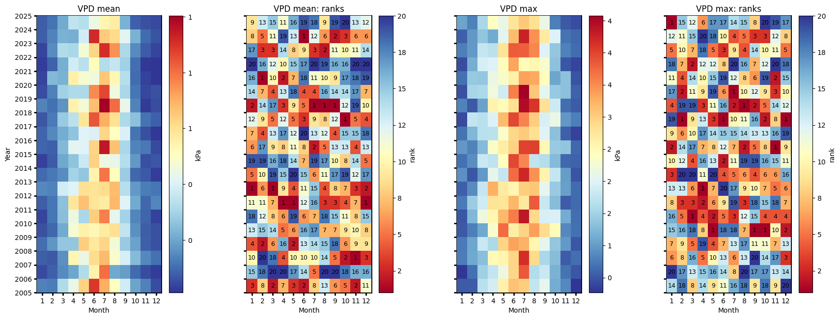
Monthly ranks

# Figure
fig = plt.figure(facecolor='white', figsize=(17, 6))

# Gridspec for layout
gs = gridspec.GridSpec(1, 4)  # rows, cols
gs.update(wspace=0.35, hspace=0.3, left=0.03, right=0.97, top=0.97, bottom=0.03)
ax_mean = fig.add_subplot(gs[0, 0])
ax_mean_ranks = fig.add_subplot(gs[0, 1])
ax_max = fig.add_subplot(gs[0, 2])
ax_max_ranks = fig.add_subplot(gs[0, 3])
params = {'axlabels_fontsize': 10, 'ticks_labelsize': 10, 'cb_labelsize': 10}
dv.heatmapyearmonth_ranks(ax=ax_mean, series=series, agg='mean', ranks=False, zlabel=units, cmap="RdYlBu_r", show_values=False, **params).plot()

hm_mean_ranks = dv.heatmapyearmonth_ranks(ax=ax_mean_ranks, series=series, agg='mean', show_values=True, **params)
hm_mean_ranks.plot()

dv.heatmapyearmonth_ranks(ax=ax_max, series=series, agg='max', ranks=False, zlabel=units, cmap="RdYlBu_r", show_values=False, **params).plot()
dv.heatmapyearmonth_ranks(ax=ax_max_ranks, series=series, agg='max', show_values=True, **params).plot()

ax_mean.set_title(f"{var} mean", color='black')
ax_mean_ranks.set_title(f"{var} mean: ranks", color='black')
ax_max.set_title(f"{var} max", color='black')
ax_max_ranks.set_title(f"{var} max: ranks", color='black')

ax_mean.tick_params(left=True, right=False, top=False, bottom=True,
                    labelleft=True, labelright=False, labeltop=False, labelbottom=True)
ax_mean_ranks.tick_params(left=True, right=False, top=False, bottom=True,
                   labelleft=False, labelright=False, labeltop=False, labelbottom=True)
ax_max.tick_params(left=True, right=False, top=False, bottom=True,
                     labelleft=False, labelright=False, labeltop=False, labelbottom=True)
ax_max_ranks.tick_params(left=True, right=False, top=False, bottom=True,
                     labelleft=False, labelright=False, labeltop=False, labelbottom=True)

ax_mean_ranks.set_ylabel("")
ax_max.set_ylabel("")
ax_max_ranks.set_ylabel("")

fig.show()

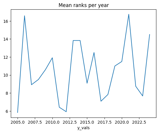
Mean ranks per year

hm_mean_ranks.hm.get_plot_data().mean(axis=1).plot(title="Mean ranks per year");

Ridgeline plots

Yearly

# rp = dv.ridgeline(series=series)
# rp.plot(
#     how='yearly',
#     kd_kwargs=None,  # params from scikit KernelDensity as dict
#     xlim=xlim,  # min/max as list
#     ylim=[0, 0.50],  # min/max as list
#     hspace=-0.8,  # overlap between months
#     xlabel=f"{var} ({units})",
#     fig_width=5,
#     fig_height=9,
#     shade_percentile=0.5,
#     show_mean_line=False,
#     fig_title=f"{var} per year (2005-2024)",
#     fig_dpi=72,
#     showplot=True,
#     ascending=False
# )

Monthly

# rp.plot(
#     how='monthly',
#     kd_kwargs=None,  # params from scikit KernelDensity as dict
#     xlim=xlim,  # min/max as list
#     ylim=[0, 0.14],  # min/max as list
#     hspace=-0.6,  # overlap between months
#     xlabel=f"{var} ({units})",
#     fig_width=4.5,
#     fig_height=8,
#     shade_percentile=0.5,
#     show_mean_line=False,
#     fig_title=f"{var} per month (2005-2024)",
#     fig_dpi=72,
#     showplot=True,
#     ascending=False
# )

Weekly

# rp.plot(
#     how='weekly',
#     kd_kwargs=None,  # params from scikit KernelDensity as dict
#     xlim=xlim,  # min/max as list
#     ylim=[0, 0.15],  # min/max as list
#     hspace=-0.6,  # overlap
#     xlabel=f"{var} ({units})",
#     fig_width=6,
#     fig_height=16,
#     shade_percentile=0.5,
#     show_mean_line=False,
#     fig_title=f"{var} per week (2005-2024)",
#     fig_dpi=72,
#     showplot=True,
#     ascending=False
# )

Single years per month

# uniq_years = series.index.year.unique()
# for uy in uniq_years:
#     series_yr = series.loc[series.index.year == uy].copy()
#     rp = dv.ridgeline(series=series_yr)
#     rp.plot(
#         how='monthly',
#         kd_kwargs=None,  # params from scikit KernelDensity as dict
#         xlim=xlim,  # min/max as list
#         ylim=[0, 0.18],  # min/max as list
#         hspace=-0.6,  # overlap
#         xlabel=f"{var} ({units})",
#         fig_width=6,
#         fig_height=7,
#         shade_percentile=0.5,
#         show_mean_line=False,
#         fig_title=f"{var} per month ({uy})",
#         fig_dpi=72,
#         showplot=True,
#         ascending=False
#     )

Single years per week

# uniq_years = series.index.year.unique()
# for uy in uniq_years:
#     series_yr = series.loc[series.index.year == uy].copy()
#     rp = dv.ridgeline(series=series_yr)
#     rp.plot(
#         how='weekly',
#         kd_kwargs=None,  # params from scikit KernelDensity as dict
#         xlim=xlim,  # min/max as list
#         ylim=[0, 0.3],  # min/max as list
#         hspace=-0.8,  # overlap
#         xlabel=f"{var} ({units})",
#         fig_width=9,
#         fig_height=18,
#         shade_percentile=0.5,
#         show_mean_line=False,
#         fig_title=f"{var} per week ({uy})",
#         fig_dpi=72,
#         showplot=True,
#         ascending=False
#     )

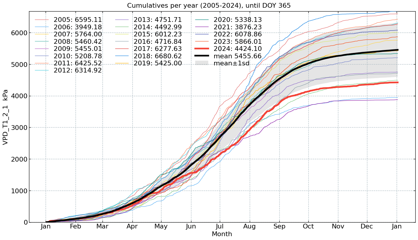
Cumulative plot

CumulativeYear(
    series=series,
    series_units=units,
    start_year=2005,
    end_year=2024,
    show_reference=True,
    excl_years_from_reference=None,
    highlight_year=2024,
    highlight_year_color='#F44336').plot();

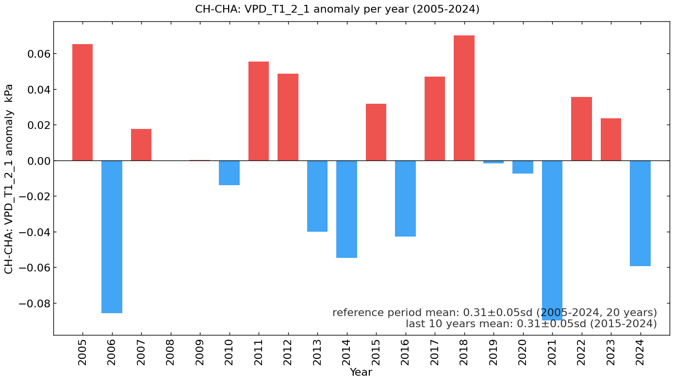
Long-term anomalies

series_yearly_mean = series.resample('YE').mean()
series_yearly_mean.index = series_yearly_mean.index.year
series_label = f"CH-CHA: {varname}"
LongtermAnomaliesYear(series=series_yearly_mean,
                      series_label=series_label,
                      series_units=units,
                      reference_start_year=2005,
                      reference_end_year=2024).plot()

End of notebook

dt_string = datetime.now().strftime("%Y-%m-%d %H:%M:%S")
print(f"Finished. {dt_string}")

Finished. 2025-05-16 13:10:31