Sonic anemometer data (2005-2024)

Modified

2 August 2026

Author: Lukas Hörtnagl (holukas@ethz.ch)

Imports

import importlib.metadata
import warnings
from datetime import datetime
from pathlib import Path
import pandas as pd
import matplotlib.pyplot as plt
import matplotlib.gridspec as gridspec

import diive as dv
from diive.core.io.files import save_parquet, load_parquet
from diive.core.plotting.cumulative import CumulativeYear
from diive.core.plotting.bar import LongtermAnomaliesYear

warnings.filterwarnings(action='ignore', category=FutureWarning)
warnings.filterwarnings(action='ignore', category=UserWarning)
version_diive = importlib.metadata.version("diive")
print(f"diive version: v{version_diive}")
diive version: v0.87.1

Load data

df75 = load_parquet(filepath=Path(r"../20_MERGE_DATA") / r"21.4_FLUXES_L1_noSHC_IRGA75+METEO7.parquet")
df72 = load_parquet(filepath=Path(r"../20_MERGE_DATA") / r"22.4_FLUXES_L1_IRGA72+METEO7_2016-2024.parquet")
Loaded .parquet file ..\20_MERGE_DATA\21.4_FLUXES_L1_noSHC_IRGA75+METEO7.parquet (2.306 seconds).
    --> Detected time resolution of <30 * Minutes> / 30min 
Loaded .parquet file ..\20_MERGE_DATA\22.4_FLUXES_L1_IRGA72+METEO7_2016-2024.parquet (1.574 seconds).
    --> Detected time resolution of <30 * Minutes> / 30min 
df72
AIR_CP AIR_DENSITY AIR_MV AIR_RHO_CP AOA_METHOD AXES_ROTATION_METHOD BADM_HEIGHTC BADM_INSTPAIR_EASTWARD_SEP_GA_CO2 BADM_INSTPAIR_EASTWARD_SEP_GA_H2O BADM_INSTPAIR_HEIGHT_SEP_GA_CO2 BADM_INSTPAIR_HEIGHT_SEP_GA_H2O BADM_INSTPAIR_NORTHWARD_SEP_GA_CO2 BADM_INSTPAIR_NORTHWARD_SEP_GA_H2O BADM_INST_AVERAGING_INT BADM_INST_GA_CP_TUBE_FLOW_RATE_GA_CO2 ... W_T_SONIC_COV_IBROM_N0004 W_T_SONIC_COV_IBROM_N0008 W_T_SONIC_COV_IBROM_N0016 W_T_SONIC_COV_IBROM_N0032 W_T_SONIC_COV_IBROM_N0065 W_T_SONIC_COV_IBROM_N0133 W_T_SONIC_COV_IBROM_N0277 W_T_SONIC_COV_IBROM_N0614 W_T_SONIC_COV_IBROM_N1626 W_UNROT W_U_COV W_VM97_TEST W_ZCD ZL ZL_UNCORR
TIMESTAMP_MIDDLE
2016-01-01 00:15:00 NaN NaN NaN NaN NaN NaN NaN NaN NaN NaN NaN NaN NaN NaN NaN ... NaN NaN NaN NaN NaN NaN NaN NaN NaN NaN NaN NaN NaN NaN NaN
2016-01-01 00:45:00 NaN NaN NaN NaN NaN NaN NaN NaN NaN NaN NaN NaN NaN NaN NaN ... NaN NaN NaN NaN NaN NaN NaN NaN NaN NaN NaN NaN NaN NaN NaN
2016-01-01 01:15:00 NaN NaN NaN NaN NaN NaN NaN NaN NaN NaN NaN NaN NaN NaN NaN ... NaN NaN NaN NaN NaN NaN NaN NaN NaN NaN NaN NaN NaN NaN NaN
2016-01-01 01:45:00 NaN NaN NaN NaN NaN NaN NaN NaN NaN NaN NaN NaN NaN NaN NaN ... NaN NaN NaN NaN NaN NaN NaN NaN NaN NaN NaN NaN NaN NaN NaN
2016-01-01 02:15:00 NaN NaN NaN NaN NaN NaN NaN NaN NaN NaN NaN NaN NaN NaN NaN ... NaN NaN NaN NaN NaN NaN NaN NaN NaN NaN NaN NaN NaN NaN NaN
... ... ... ... ... ... ... ... ... ... ... ... ... ... ... ... ... ... ... ... ... ... ... ... ... ... ... ... ... ... ... ...
2024-12-31 21:45:00 1008.09 1.20135 0.024060 1211.07 0.0 1.0 37.0 1.0 1.0 -1.0 -1.0 11.0 11.0 30.0 12.0 ... 0.011309 0.009592 0.007451 0.005559 0.004089 0.003105 0.002487 0.002084 0.001849 -0.138079 0.016036 800000000.0 21.0 -0.178429 -0.179257
2024-12-31 22:15:00 1008.14 1.20010 0.024085 1209.87 0.0 1.0 37.0 1.0 1.0 -1.0 -1.0 11.0 11.0 30.0 12.0 ... 0.030220 0.037705 0.044831 0.050684 0.054646 0.056600 0.057335 0.057556 0.057558 -0.005790 -0.118170 800000000.0 8.0 -0.316167 -0.321022
2024-12-31 22:45:00 1008.20 1.20023 0.024081 1210.07 0.0 1.0 37.0 1.0 1.0 -1.0 -1.0 11.0 11.0 30.0 12.0 ... 0.030814 0.034314 0.037230 0.040106 0.042843 0.045204 0.046974 0.048092 0.048710 0.065927 -0.196501 800000000.0 9.0 -0.101105 -0.102196
2024-12-31 23:15:00 1008.19 1.19504 0.024186 1204.83 0.0 1.0 37.0 1.0 1.0 -1.0 -1.0 11.0 11.0 30.0 12.0 ... 0.014113 -0.000404 -0.008502 -0.010467 -0.011853 -0.012772 -0.012849 -0.012584 -0.012387 0.115006 -0.316383 800000000.0 3.0 -0.051475 -0.052922
2024-12-31 23:45:00 1008.15 1.20042 0.024078 1210.20 0.0 1.0 37.0 1.0 1.0 -1.0 -1.0 11.0 11.0 30.0 12.0 ... -0.009548 -0.012178 -0.013227 -0.014364 -0.015350 -0.015919 -0.016282 -0.016600 -0.016840 -0.087622 0.098774 800000000.0 10.0 0.049339 0.049809

157824 rows × 342 columns

# xlabel = f"{var} ({units})"
# xlim = [series.min(), series.max()]


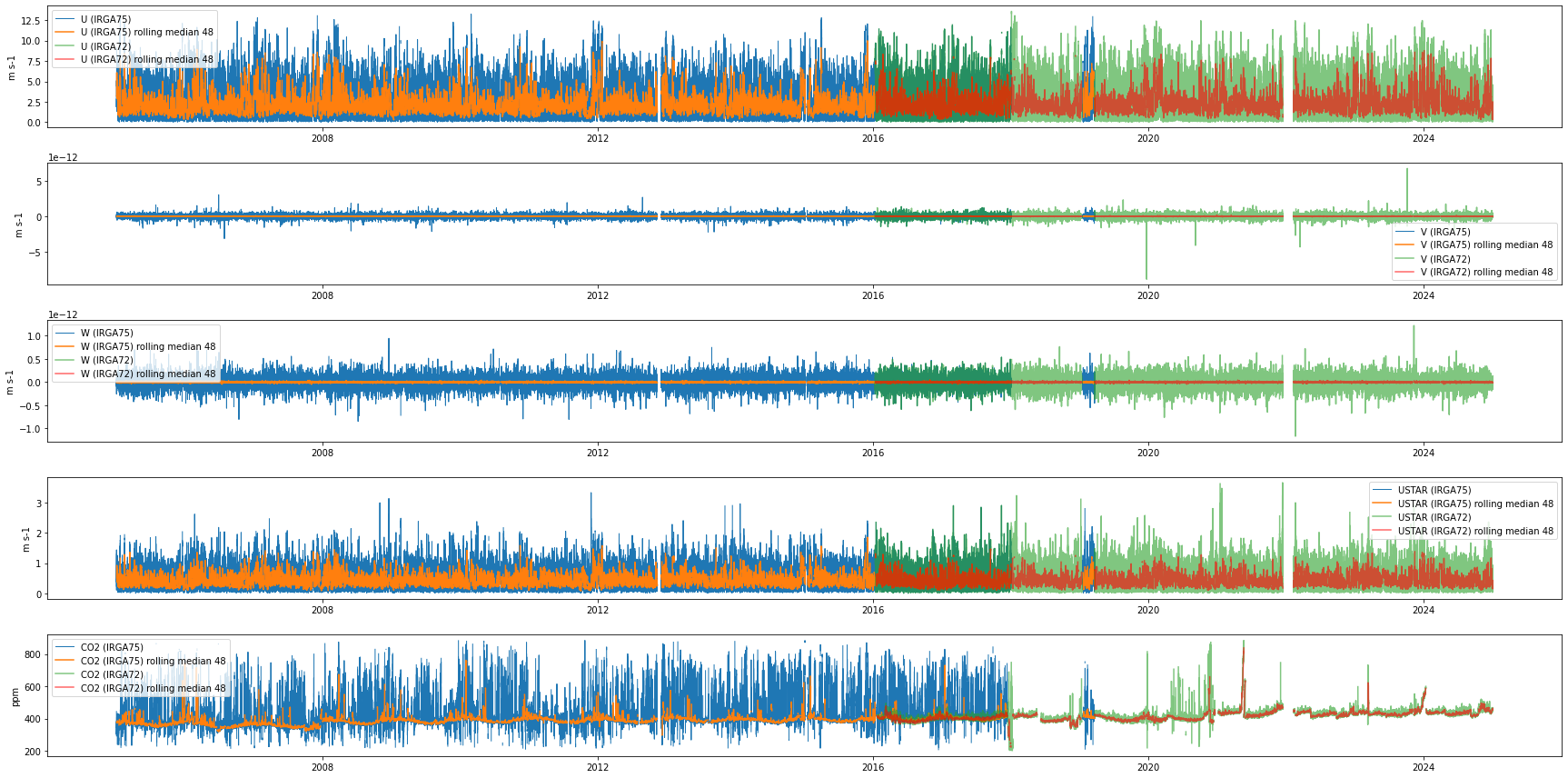
Wind comparison

import pandas as pd
import matplotlib.pyplot as plt
import numpy as np

def plot(var, ax, ylabel):
    windowsize = 48
    s1 = df75[var]
    s2 = df72[var]
    # axes[ax].set_title(var)
    axes[ax].plot(s1, label=f'{var} (IRGA75)', lw=1)
    axes[ax].plot(s1.rolling(window=windowsize, min_periods=windowsize).median(), label=f'{var} (IRGA75) rolling median {windowsize}')
    axes[ax].plot(s2, label=f'{var} (IRGA72)', alpha=.6)
    axes[ax].plot(s2.rolling(window=windowsize, min_periods=windowsize).median(), label=f'{var} (IRGA72) rolling median {windowsize}', color='red', alpha=.6)
    axes[ax].set_ylabel(ylabel)
    axes[ax].legend()

# Create a figure with two subplots arranged vertically
fig, axes = plt.subplots(5, 1, figsize=(24, 12), dpi=72)
# axes[1].sharey(axes[0])
plot(var='U', ax=0, ylabel='m s-1')
plot(var='V', ax=1, ylabel='m s-1')
plot(var='W', ax=2, ylabel='m s-1')
plot(var='USTAR', ax=3, ylabel='m s-1')
plot(var='CO2', ax=4, ylabel='ppm')

plt.tight_layout()

import pandas as pd
import matplotlib.pyplot as plt
import numpy as np

def plot(var, ax, ylabel):
    windowsize = 48
    s1 = df75[var]
    s2 = df72[var]
    # axes[ax].set_title(var)
    axes[ax].plot(s1, label=f'{var} (IRGA75)', lw=1)
    axes[ax].plot(s1.rolling(window=windowsize, min_periods=windowsize).median(), label=f'{var} (IRGA75) rolling median {windowsize}')
    axes[ax].plot(s2, label=f'{var} (IRGA72)', alpha=.6)
    axes[ax].plot(s2.rolling(window=windowsize, min_periods=windowsize).median(), label=f'{var} (IRGA72) rolling median {windowsize}', color='red', alpha=.6)
    axes[ax].set_ylabel(ylabel)
    axes[ax].legend()

# Create a figure with two subplots arranged vertically
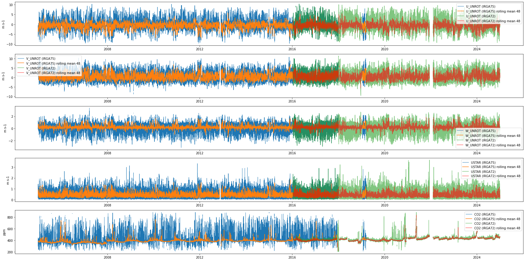
fig, axes = plt.subplots(5, 1, figsize=(24, 12), dpi=72)
# axes[1].sharey(axes[0])
plot(var='U_UNROT', ax=0, ylabel='m s-1')
plot(var='V_UNROT', ax=1, ylabel='m s-1')
plot(var='W_UNROT', ax=2, ylabel='m s-1')
plot(var='USTAR', ax=3, ylabel='m s-1')
plot(var='CO2', ax=4, ylabel='ppm')

plt.tight_layout()

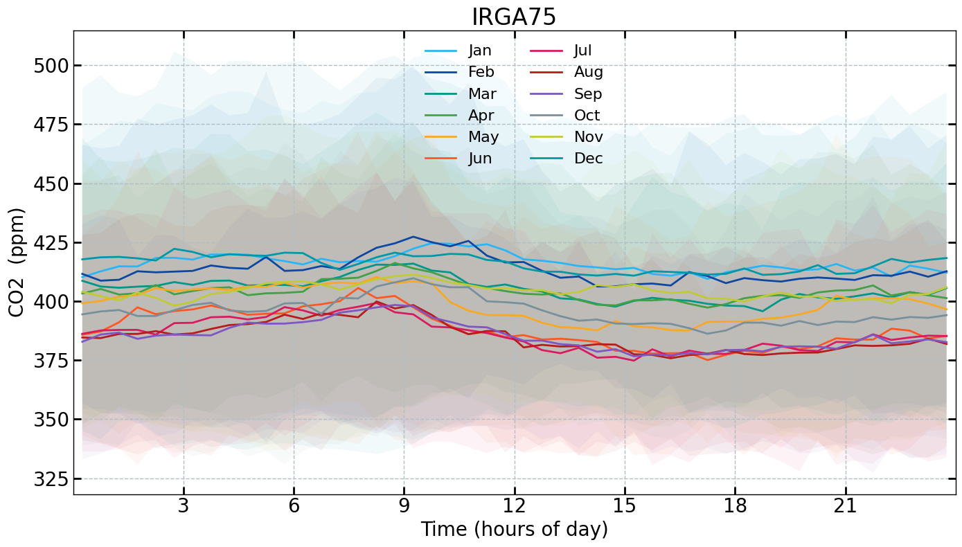
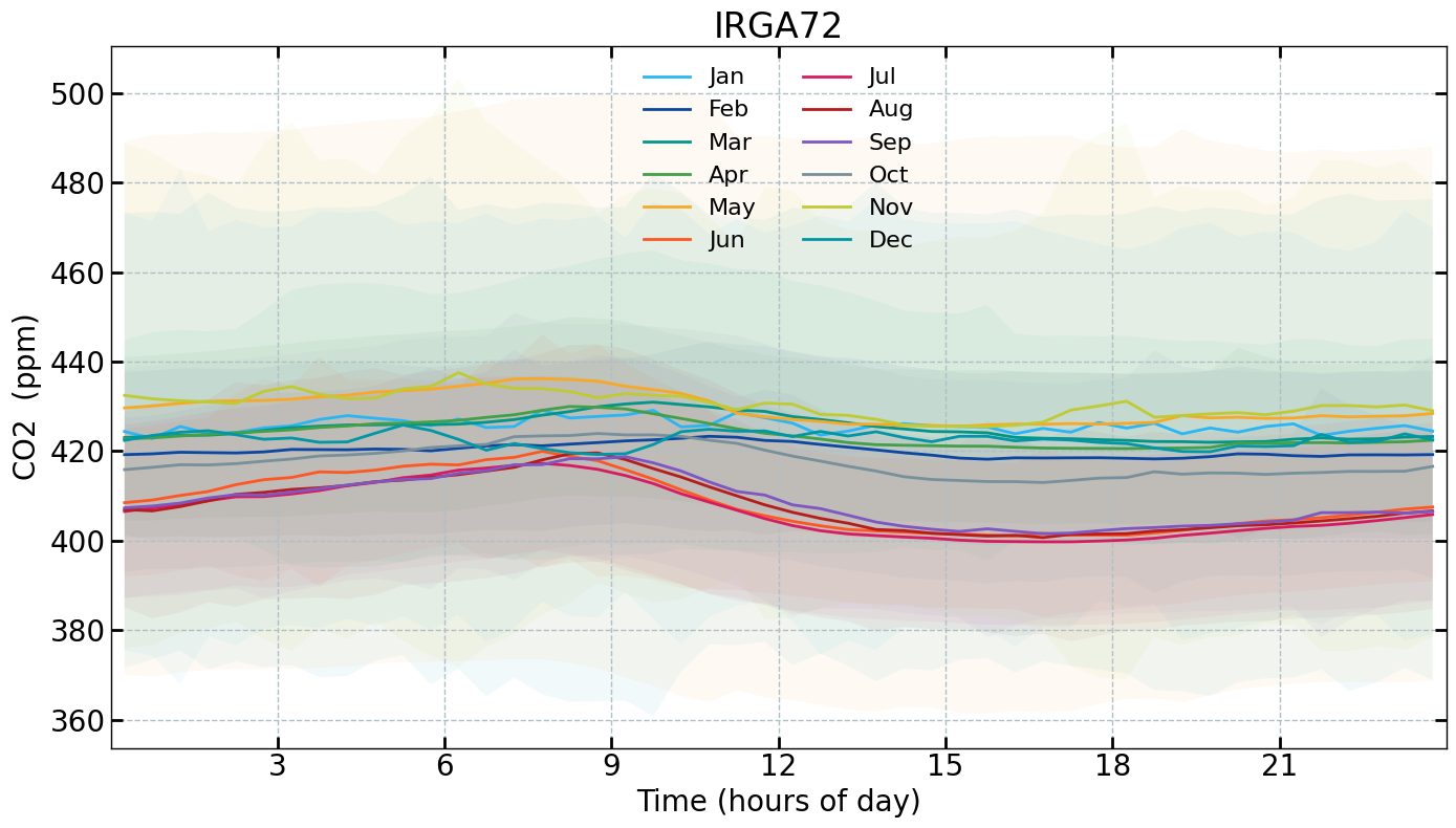
CO2 comparison

from diive.core.plotting.dielcycle import DielCycle
title = r'$\mathrm{Mean\ CO_2}$'
units = r'($\mathrm{ppm}$)'
each_month = True

dc = DielCycle(series=df75['CO2'])
dc.plot(title="IRGA75", txt_ylabel_units=units, each_month=each_month, legend_n_col=2);

dc = DielCycle(series=df72['CO2'])
dc.plot(title="IRGA72", txt_ylabel_units=units, each_month=each_month, legend_n_col=2);

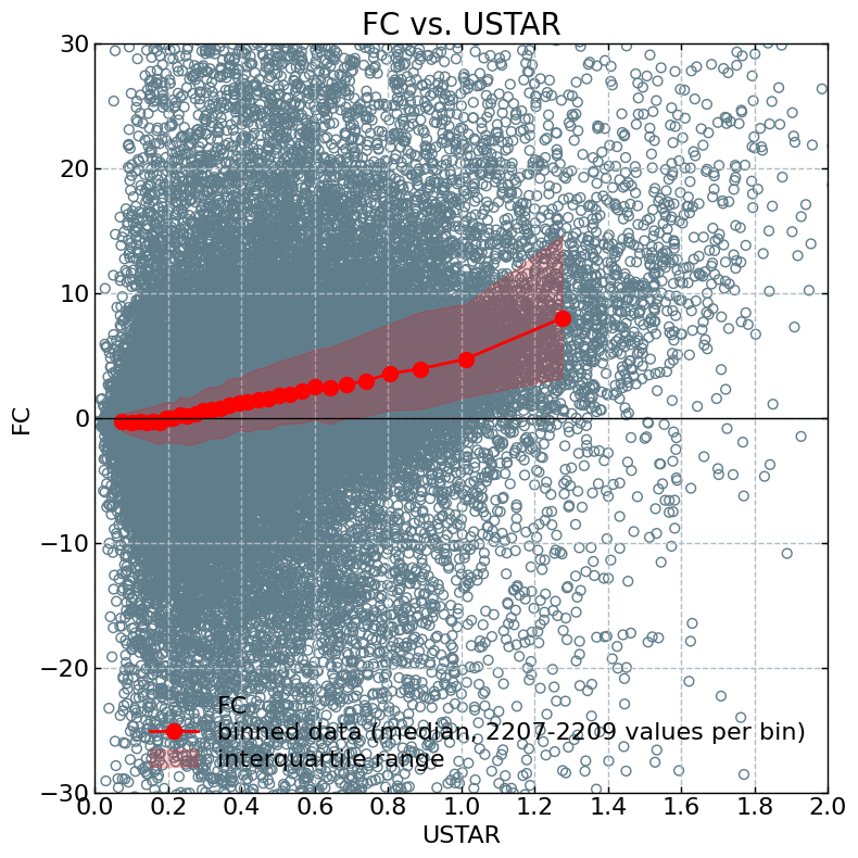
FC vs nighttime USTAR

subset75 = df75.loc[(df75['SW_IN_POT'] < 20) & (df75['FC_SSITC_TEST'] <= 1) & (df75['FC'] >= -50) & (df75['FC'] <= 50), ['USTAR', 'FC']]
from diive.core.plotting.scatter import ScatterXY
x = subset75['USTAR']
y = subset75['FC']
ScatterXY(x=x, y=y, nbins=30, xlim=[0, 2], ylim=[-30, 30]).plot();
# plt.scatter(subset75['USTAR'], subset75['FC'], alpha=.01)

# [print(c) for c in df75.columns if "SSITC" in c];
ET_SSITC_TEST
FC_SSITC_TEST
FH2O_SSITC_TEST
H_SSITC_TEST
LE_SSITC_TEST
TAU_SSITC_TEST

Stats

Overall mean

_yearly_avg = series.resample('YE').mean()
_overall_mean = _yearly_avg.mean()
_overall_sd = _yearly_avg.std()
print(f"Overall mean: {_overall_mean} +/- {_overall_sd}")
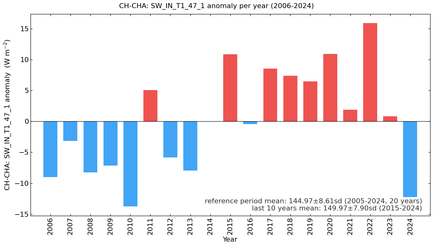
Overall mean: 144.96503741344142 +/- 8.608602956557682

Yearly means

series.resample('YE').mean()
TIMESTAMP_MIDDLE
2006-12-31    135.939501
2007-12-31    141.805157
2008-12-31    136.728011
2009-12-31    137.843690
2010-12-31    131.191375
2011-12-31    150.020200
2012-12-31    139.144684
2013-12-31    137.017228
2014-12-31    144.983657
2015-12-31    155.818257
2016-12-31    144.510632
2017-12-31    153.484954
2018-12-31    152.331358
2019-12-31    151.435834
2020-12-31    155.872297
2021-12-31    146.824263
2022-12-31    160.850230
2023-12-31    145.794347
2024-12-31    132.740037
Freq: YE-DEC, Name: SW_IN_T1_47_1, dtype: float64

Monthly averages

seriesdf = pd.DataFrame(series)
seriesdf['MONTH'] = seriesdf.index.month
seriesdf['YEAR'] = seriesdf.index.year
monthly_avg = seriesdf.groupby(['YEAR', 'MONTH'])[varname].mean().unstack()
monthly_avg
MONTH 1 2 3 4 5 6 7 8 9 10 11 12
YEAR
2006 50.899051 58.722736 106.317192 162.769202 189.103795 268.566624 284.475316 146.286217 155.189567 100.150799 64.252037 40.742373
2007 39.825179 77.110025 135.987100 253.702291 212.135527 227.360596 219.522755 182.137087 163.059730 103.842508 51.798866 33.005676
2008 48.027879 106.239409 117.438274 139.057256 241.774568 227.176324 243.220083 203.113396 139.387541 90.250120 53.999669 29.605070
2009 39.537355 76.455523 105.414743 200.706655 229.433903 252.546844 227.345487 196.290979 160.682545 96.251005 48.490726 29.682786
2010 37.227410 67.457293 126.035488 213.073504 161.499327 222.754495 239.540399 176.939965 167.063098 91.224560 48.279606 28.940100
2011 40.045098 76.125026 143.873194 239.485702 269.005390 209.502899 230.267809 236.678244 170.655131 96.865746 56.093205 27.286685
2012 34.772823 97.623528 174.426550 146.489266 243.958609 233.521002 226.440464 212.188406 149.568234 73.956370 42.192407 33.467133
2013 40.008816 60.714161 102.239948 142.963816 183.008096 240.358686 290.239942 232.297106 153.324410 86.207134 44.734129 63.983770
2014 45.105636 81.426023 163.471591 189.202980 217.711388 294.751177 195.611411 193.154618 162.935567 102.434049 61.204169 30.687367
2015 42.647671 79.779470 148.627451 220.482235 209.283441 262.058698 290.020636 229.934124 166.635166 88.526500 70.027535 57.957903
2016 28.495295 60.516284 126.481138 174.018331 210.238603 210.514726 256.641640 241.095892 188.522970 97.610462 50.726758 57.771249
2017 43.287703 90.370013 157.229064 197.213344 252.457034 287.077811 239.670439 221.172415 154.763591 120.414591 43.891647 30.389918
2018 37.885127 61.582151 113.197964 227.988522 222.078713 267.702677 272.618518 230.696239 191.190187 120.990314 49.198602 28.259290
2019 42.236491 113.767870 148.763149 175.596706 196.894817 279.076977 282.542682 221.527967 177.367912 91.534162 21.901103 37.987930
2020 59.350377 81.074998 154.084398 253.454911 249.777637 225.567435 276.231263 217.614880 173.808747 86.153202 61.039162 30.400444
2021 37.137552 97.099087 150.740700 225.867687 205.033384 255.626630 213.779638 194.454147 187.962766 117.440944 45.184148 30.390747
2022 59.536808 98.149522 178.366098 203.498698 253.611379 272.680898 294.516460 240.028843 144.042191 99.652736 50.471514 30.460197
2023 34.255274 94.977668 116.150278 152.859156 209.189453 309.442907 249.589123 202.361234 196.844986 110.799587 37.855937 34.773226
2024 44.343884 76.217271 122.114467 160.926099 193.128574 209.619923 245.619367 239.003301 144.914168 75.141472 46.783186 35.197507


Heatmap plots

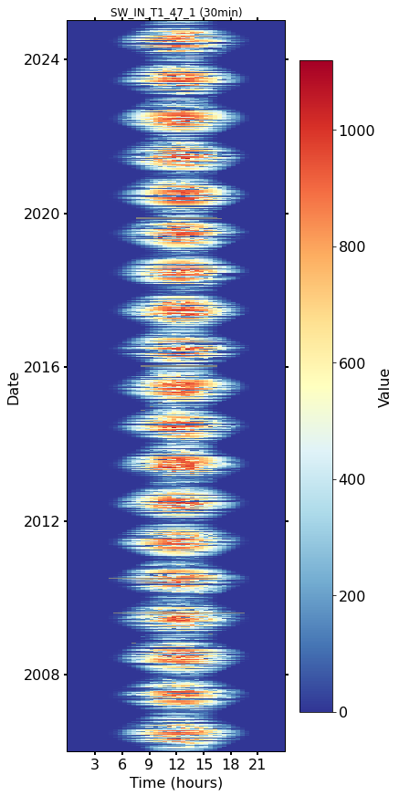
Half-hourly

fig, axs = plt.subplots(ncols=1, figsize=(6, 12), dpi=72, layout="constrained")
dv.heatmapdatetime(series=series, ax=axs, cb_digits_after_comma=0).plot()

Monthly

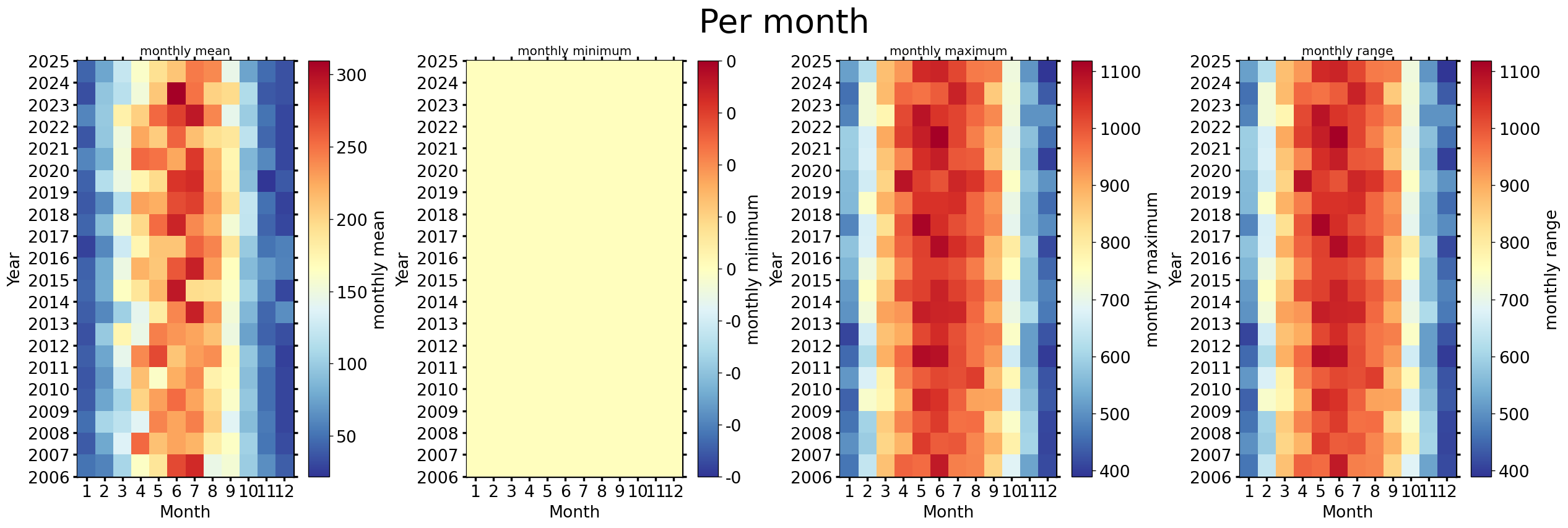
fig, axs = plt.subplots(ncols=4, figsize=(21, 7), dpi=120, layout="constrained")
fig.suptitle(f'Per month', fontsize=32)
dv.heatmapyearmonth(series_monthly=series.resample('M').mean(), title="monthly mean", ax=axs[0], cb_digits_after_comma=0, zlabel="monthly mean").plot()
dv.heatmapyearmonth(series_monthly=series.resample('M').min(), title="monthly minimum", ax=axs[1], cb_digits_after_comma=0, zlabel="monthly minimum").plot()
dv.heatmapyearmonth(series_monthly=series.resample('M').max(), title="monthly maximum", ax=axs[2], cb_digits_after_comma=0, zlabel="monthly maximum").plot()
_range = series.resample('M').max().sub(series.resample('M').min())
dv.heatmapyearmonth(series_monthly=_range, title="monthly range", ax=axs[3], cb_digits_after_comma=0, zlabel="monthly range").plot()

Monthly ranks

# Figure
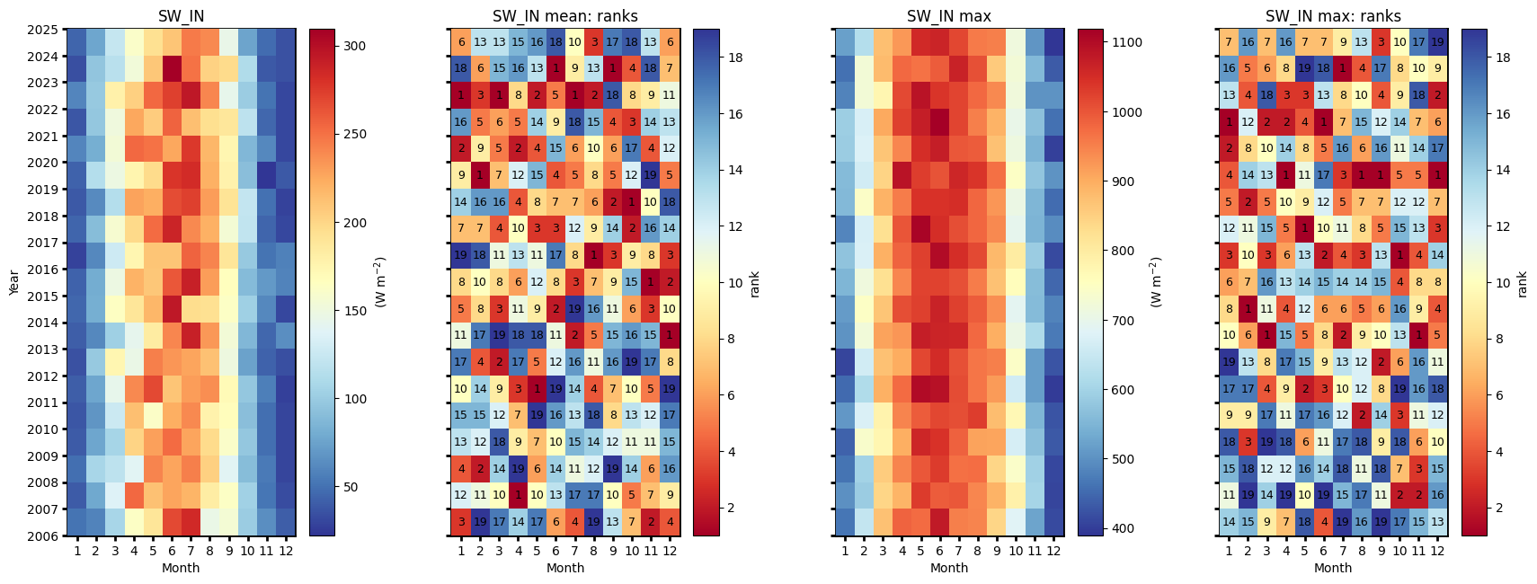
fig = plt.figure(facecolor='white', figsize=(17, 6))

# Gridspec for layout
gs = gridspec.GridSpec(1, 4)  # rows, cols
gs.update(wspace=0.35, hspace=0.3, left=0.03, right=0.97, top=0.97, bottom=0.03)
ax_mean = fig.add_subplot(gs[0, 0])
ax_mean_ranks = fig.add_subplot(gs[0, 1])
ax_max = fig.add_subplot(gs[0, 2])
ax_max_ranks = fig.add_subplot(gs[0, 3])
params = {'axlabels_fontsize': 10, 'ticks_labelsize': 10, 'cb_labelsize': 10}
dv.heatmapyearmonth_ranks(ax=ax_mean, series=series, agg='mean', ranks=False, zlabel=f"{units}", cmap="RdYlBu_r", show_values=False, **params).plot()

hm_mean_ranks = dv.heatmapyearmonth_ranks(ax=ax_mean_ranks, series=series, agg='mean', **params)
hm_mean_ranks.plot()

dv.heatmapyearmonth_ranks(ax=ax_max, series=series, agg='max', ranks=False, zlabel=f"{units}", cmap="RdYlBu_r", show_values=False, **params).plot()
dv.heatmapyearmonth_ranks(ax=ax_max_ranks, series=series, agg='max', **params).plot()

ax_mean.set_title(f"{var}", color='black')
ax_mean_ranks.set_title(f"{var} mean: ranks", color='black')
ax_max.set_title(f"{var} max", color='black')
ax_max_ranks.set_title(f"{var} max: ranks", color='black')

ax_mean.tick_params(left=True, right=False, top=False, bottom=True,
                    labelleft=True, labelright=False, labeltop=False, labelbottom=True)
ax_mean_ranks.tick_params(left=True, right=False, top=False, bottom=True,
                   labelleft=False, labelright=False, labeltop=False, labelbottom=True)
ax_max.tick_params(left=True, right=False, top=False, bottom=True,
                     labelleft=False, labelright=False, labeltop=False, labelbottom=True)
ax_max_ranks.tick_params(left=True, right=False, top=False, bottom=True,
                     labelleft=False, labelright=False, labeltop=False, labelbottom=True)

ax_mean_ranks.set_ylabel("")
ax_max.set_ylabel("")
ax_max_ranks.set_ylabel("")

fig.show()
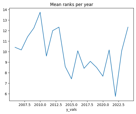
Mean ranks per year

hm_mean_ranks.hm.get_plot_data().mean(axis=1).plot(title="Mean ranks per year");


Ridgeline plots

Yearly

# rp = dv.ridgeline(series=series)
# rp.plot(
#     how='yearly',
#     kd_kwargs=None,  # params from scikit KernelDensity as dict
#     xlim=xlim,  # min/max as list
#     ylim=[0, 0.01],  # min/max as list
#     hspace=-0.8,  # overlap between months
#     xlabel=f"{var} ({units})",
#     fig_width=5,
#     fig_height=9,
#     shade_percentile=0.5,
#     show_mean_line=False,
#     fig_title=f"{var} per year (2005-2024)",
#     fig_dpi=72,
#     showplot=True,
#     ascending=False
# )

Monthly

# rp.plot(
#     how='monthly',
#     kd_kwargs=None,  # params from scikit KernelDensity as dict
#     xlim=xlim,  # min/max as list
#     ylim=[0, 0.01],  # min/max as list
#     hspace=-0.6,  # overlap between months
#     xlabel=f"{var} ({units})",
#     fig_width=4.5,
#     fig_height=8,
#     shade_percentile=0.5,
#     show_mean_line=False,
#     fig_title=f"{var} per month (2005-2024)",
#     fig_dpi=72,
#     showplot=True,
#     ascending=False
# )

Weekly

# rp.plot(
#     how='weekly',
#     kd_kwargs=None,  # params from scikit KernelDensity as dict
#     xlim=xlim,  # min/max as list
#     ylim=[0, 0.15],  # min/max as list
#     hspace=-0.6,  # overlap
#     xlabel=f"{var} ({units})",
#     fig_width=6,
#     fig_height=16,
#     shade_percentile=0.5,
#     show_mean_line=False,
#     fig_title=f"{var} per week (2005-2024)",
#     fig_dpi=72,
#     showplot=True,
#     ascending=False
# )

Single years per month

# uniq_years = series.index.year.unique()
# for uy in uniq_years:
#     series_yr = series.loc[series.index.year == uy].copy()
#     rp = dv.ridgeline(series=series_yr)
#     rp.plot(
#         how='monthly',
#         kd_kwargs=None,  # params from scikit KernelDensity as dict
#         xlim=xlim,  # min/max as list
#         ylim=[0, 0.18],  # min/max as list
#         hspace=-0.6,  # overlap
#         xlabel=f"{var} ({units})",
#         fig_width=6,
#         fig_height=7,
#         shade_percentile=0.5,
#         show_mean_line=False,
#         fig_title=f"{var} per month ({uy})",
#         fig_dpi=72,
#         showplot=True,
#         ascending=False
#     )

Single years per week

# uniq_years = series.index.year.unique()
# for uy in uniq_years:
#     series_yr = series.loc[series.index.year == uy].copy()
#     rp = dv.ridgeline(series=series_yr)
#     rp.plot(
#         how='weekly',
#         kd_kwargs=None,  # params from scikit KernelDensity as dict
#         xlim=xlim,  # min/max as list
#         ylim=[0, 0.3],  # min/max as list
#         hspace=-0.8,  # overlap
#         xlabel=f"{var} ({units})",
#         fig_width=9,
#         fig_height=18,
#         shade_percentile=0.5,
#         show_mean_line=False,
#         fig_title=f"{var} per week ({uy})",
#         fig_dpi=72,
#         showplot=True,
#         ascending=False
#     )


Cumulative plot

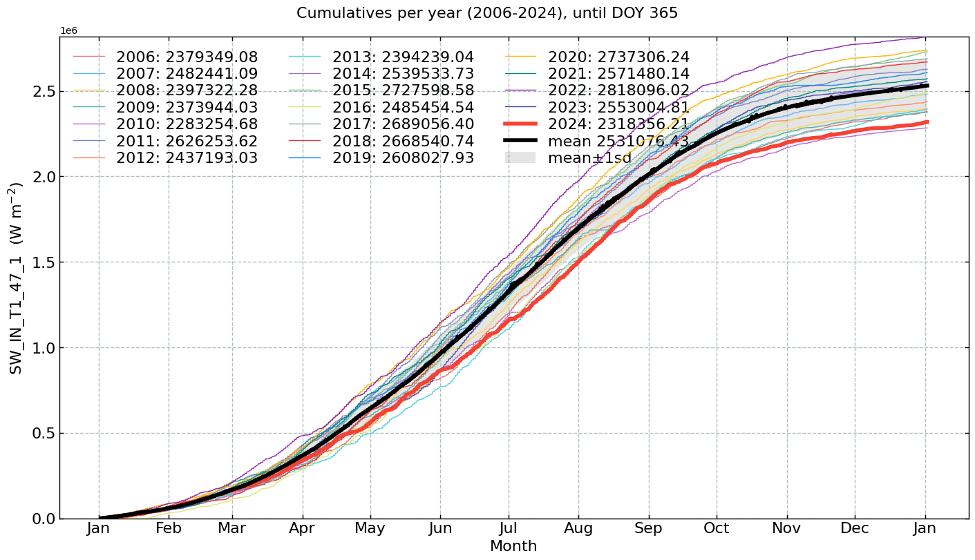
CumulativeYear(
    series=series,
    series_units=units,
    start_year=2005,
    end_year=2024,
    show_reference=True,
    excl_years_from_reference=None,
    highlight_year=2024,
    highlight_year_color='#F44336').plot();


Long-term anomalies

series_yearly_mean = series.resample('YE').mean()
series_yearly_mean.index = series_yearly_mean.index.year
series_label = f"CH-CHA: {varname}"
LongtermAnomaliesYear(series=series_yearly_mean,
                      series_label=series_label,
                      series_units=units,
                      reference_start_year=2005,
                      reference_end_year=2024).plot()


End of notebook

dt_string = datetime.now().strftime("%Y-%m-%d %H:%M:%S")
print(f"Finished. {dt_string}")
Finished. 2025-06-11 22:13:59
Back to top